Finite Difference Method for Elliptic PDEs

Section 4.10 Finite Difference Method for Elliptic PDEs

Subsection 4.10.1 Examples of Elliptic PDEs

Elliptic PDE’s are equations with second derivatives in space and no time derivative. The most important examples are Laplace’s equation

\begin{equation*} \Delta u = u_{xx}+ u_{yy}+ u_{zz}= 0 \end{equation*}

and the Poisson equation

\begin{equation*} \Delta u = f(x,y,z)\text{.} \end{equation*}

These equations are used in a large variety of steady-state physical situations such as: steady state heat problems, steady state chemical distributions, electrostatic potentials, elastic deformation and steady state fluid flows.

🔗

For the sake of clarity we will only consider the two dimensional problem. A good model problem in this dimension is the elastic deflection of a membrane. Suppose that a membrane such as a sheet of rubber is stretched across a rectangular frame. If some of the edges of the frame are bent, or if forces are applied to the sheet then it will deflect by an amount \(u(x,y)\) at each point \((x,y)\text{.}\) This \(u\) will satisfy the boundary value problem:

\begin{equation} \begin{split}u_{xx}+ u_{yy}&= f(x,y) \quad\text{for}\quad (x,y) \text{ in }R, \\ u(x,y)&= g(x,y) \quad\text{for}\quad (x,y) \text{ on }\partial R\end{split}\text{,}\tag{4.10.1} \end{equation}

where \(R\) is the rectangle, \(\partial R\) is the edge of the rectangle, \(f(x,y)\) is the force density (pressure) applied at each point and \(g(x,y)\) is the deflection at the edge.

🔗

Subsection 4.10.2 The Finite Difference Equations

Suppose the rectangle is described by

\begin{equation*} R = \{ a\le x \le b, c \le y \le d\}\text{.} \end{equation*}

We will divide \(R\) in sub-rectangles. If we have \(m\) subdivisions in the \(x\) direction and \(n\) subdivisions in the \(y\) direction, then the step size in the \(x\) and \(y\) directions respectively are

\begin{equation*} h = \frac{b-a}{m}\quad \text{and}\quad k = \frac{d-c}{n}\text{.} \end{equation*}

We obtain the finite difference equations for (4.10.1) by replacing \(u_{xx}\) and \(u_{yy}\) by their central differences to obtain

\begin{equation} \frac{u_{i+1,j}- 2u_{ij}+ u_{i-1,j}}{h^{2}}+ \frac{u_{i,j+1}- 2u_{ij}+ u_{i,j-1}}{k^{2}}= f(x_{i},y_{j}) = f_{ij}\tag{4.10.2} \end{equation}

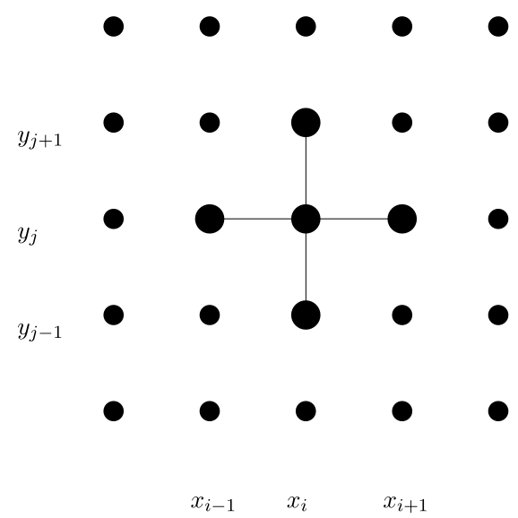
for \(1 \le i \le m-1\) and \(1 \le j \le n-1\text{.}\) See Figure 4.10.1 for an illustration. The boundary conditions are introduced by

\begin{align} u_{0,j} \amp = g(a,y_{j}),\tag{4.10.3}\\ u_{m,j} \amp = g(b,y_{j}),\notag\\ u_{i,0} \amp = g(x_{i},c), \quad\text{and}\notag\\ u_{i,n} \amp = g(x_{i},d)\text{.}\notag \end{align}

🔗

Schematic of elliptic finite difference.🔗 — Figure 4.10.1. The finite difference equation relates five neighboring values in a \(+\) pattern.
🔗

🔗

Subsection 4.10.3 Direct Solution of the Equations

Notice that since the edge values are prescribed, there are \((m-1) \times (n-1)\) grid points where we need to determine the solution. Note also that there are exactly \((m-1) \times (n-1)\) equations in (4.10.2). Finally, notice that the equations are all linear. Thus we could solve the equations exactly using matrix methods. To do this we would first need to express the \(u_{ij}\)’s as a vector, rather then a matrix. To do this there is a standard procedure: let \(\ub\) be the column vector we get by placing one column after another from the columns of \((u_{ij})\text{.}\) Thus we would list \(u_{:,1}\) first then \(u_{:,2}\text{,}\) etc.. Next we would need to write the matrix \(A\) that contains the coefficients of the equations (4.10.2) and incorporate the boundary conditions in a vector \(\bb\text{.}\) Then we could solve an equation of the form

\begin{equation} A \ub = \bb\text{.}\tag{4.10.4} \end{equation}

Setting up and solving this equation is called the direct method.

🔗

An advantage of the direct method is that solving (4.10.4) can be done relatively quickly and accurately. The drawback of the direct method is that one must set up \(\ub\text{,}\) \(A\) and \(\bb\text{,}\) which is confusing. Further, the matrix \(A\) has dimensions \((m-1)(n-1) \times (m-1)(n-1)\text{,}\) which can be rather large. Although \(A\) is large, many of its elements are zero. Such a matrix is called sparse and there are special methods intended for efficiently working with sparse matrices.

🔗

Subsection 4.10.4 Iterative Solution

A usually preferred alternative to the direct method described above is to solve the finite difference equations iteratively. To do this, first solve (4.10.2) for \(u_{ij}\text{,}\) which yields

\begin{equation*} u_{ij}= \frac{1}{2(h^{2}+k^{2})}\left( k^{2} (u_{i+1,j}+ u_{i-1,j}) + h^{2} (u_{i,j+1}+ u_{i,j-1}) - h^{2} k^{2} f_{ij}\right) \text{.} \end{equation*}

This method is another example of a relaxation method. Using this formula, along with (4.10.3), we can update \(u_{ij}\) from its neighbors, just as we did in the relaxation method for the nonlinear boundary value problem. If this method converges, then the result is an approximate solution.

🔗

Download and read the script mypoisson.m (Program A.2.7), which implements the iterative solution. You will notice that maxit is set to \(0\text{.}\) Thus the program will not do any iteration, but will plot the initial guess. The initial guess in this case consists of the proper boundary values at the edges, and zero everywhere in the interior. To see the solution evolve, gradually increase maxit.

🔗

Exercises 4.10.5 Exercises

1.

Modify the script mypoisson.m (Program A.2.7) to change the force \(f(x,y)\) to a negative constant \(-p\text{.}\)

🔗

Obtain plots for \(p=5\) and \(p=50\text{.}\) You will need to adjust maxit to obtain convergence. Tell how many iterations are needed for convergence in each. Turn in your plots and the modified program.

🔗

2.

Further modify mypoisson.m (Program A.2.7) to change the edge of the rectangle at \(x = b \ (= 10)\) to be an insulated boundary, i.e. \(u_{x}(b,y) =0\text{.}\)

🔗

You will need to expand both the grid and the matrix u to include a row of fictional points. Then you will need to adjust a lot of indices and enforce insulation inside the loop. Run it with \(p = 20\text{.}\) If it is working correctly, the plot will be smooth and the derivative \(u_{x}\) on the edge \(x = 10\) will appear to be zero. Turn in your plots and the modified program.

🔗

Prev Top Next