Double Integrals for Rectangles

Section 3.7 Double Integrals for Rectangles

Subsection 3.7.1 The center point method

Suppose that we need to find the integral of a function, \(f(x,y)\text{,}\) on a rectangle

\begin{equation*} R = \{(x,y): a\le x \le b, c \le y \le d\}\text{.} \end{equation*}

Calculus tells us to do this by an iterated integral

\begin{equation*} I = \iint_{R} f \, dA = \int_{a}^{b} \int_{c}^{d} f(x,y) \, dy dx = \int_{c}^{d} \int_{a}^{b} f(x,y) \, dx dy\text{.} \end{equation*}

For instance, if \(R\) is the rectangle \(0 \le x \le 2\text{,}\) \(1 \le y \le 3\text{,}\) then

\begin{equation*} \begin{split}\iint_{R} x^{2} y \, dA&= \int_{0}^{2} \left(\int_{1}^{3} x^{2} y \, dy \right) \, dx \\&= \int_{0}^{2} x^{2} \left(\left. \frac{y^{2}}{2}\right|_{1}^{3} \right) \, dx \\&= \int_{0}^{2} x^{2} \left( \frac{9}{2}- \frac{1}{2}\right) \, dx \\&= 4 \int_{0}^{2} x^{2} \, dx\\&= 4 \cdot \frac{8}{3}= \frac{32}{3}= 10.66... .\end{split} \end{equation*}

Calculus also tells us that the integral is the limit of the Riemann sums of the function as the size of the subrectangles goes to zero. This means that the Riemann sums are approximations of the integral, which is precisely what we need for numerical methods.

🔗

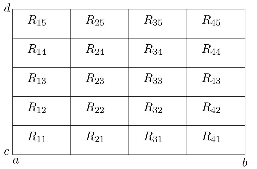
For a rectangle \(R\text{,}\) we begin by subdividing into smaller subrectangles \(\{R_{ij}\}\text{,}\) in a systematic way. We will divide \([a,b]\) into \(m\) subintervals and \([c,d]\) into \(n\) subintervals. Then \(R_{ij}\) will be the “intersection” of the \(i\)-th subinterval in \([a,b]\) with the \(j\)-th subinterval of \([c,d]\text{.}\) In this way the entire rectangle is subdivided into \(mn\) subrectangles, numbered as in Figure Figure 3.7.1.

🔗

Diagram of a rectangle subdivided into 5 x 4 rectangles.🔗 — Figure 3.7.1. Subdivision of the rectangle \(R = [a,b] \times [c,d]\) into subrectangles \(R_{ij}\text{.}\) Note that the arrangement in the \(x\)-\(y\) plane is completely different from the convention in a matrix.
🔗

A Riemann sum using this subdivision would have the form

\begin{equation*} S = \sum_{i,j=1,1}^{m,n}f(x^{*}_{ij}) A_{ij}= \sum_{j=1}^{n} \left(\sum_{i=1}^{m} f(x^{*}_{ij}) A_{ij}\right)\text{,} \end{equation*}

where \(A_{ij}= \Delta x_{i} \Delta y_{j}\) is the area of \(R_{ij}\text{,}\) and \(x^{*}_{ij}\) is a point in \(R_{ij}\text{.}\) The theory of integrals tells us that if \(f\) is continuous, then this sum will converge to the same number, no matter how we choose \(x^{*}_{ij}\text{.}\) For instance, we could choose \(x^{*}_{ij}\) to be the point in the lower left corner of \(R_{ij}\) and the sum would still converge as the size of the subrectangles goes to zero. However, in practice we wish to choose \(x^{*}_{ij}\) in such a way to make \(S\) as accurate as possible even when the subrectangles are not very small. The obvious choice for the best point in \(R_{ij}\) would be the center point. The center point is most likely of all points to have a value of \(f\) close to the average value of \(f\text{.}\) If we denote the center points by \(c_{ij}\text{,}\) then the sum becomes

\begin{equation*} C_{mn}= \sum_{i,j=1,1}^{m,n}f(c_{ij}) A_{ij}\text{.} \end{equation*}

Here

\begin{equation*} c_{ij}= \left( \frac{x_{i-1}+ x_{i}}{2}, \frac{y_{i-1}+ y_{i}}{2}\right)\text{.} \end{equation*}

Note that if the subdivision is evenly spaced then \(\Delta x \equiv (b-a)/m\) and \(\Delta y \equiv (d-c)/n\text{,}\) and so in that case

\begin{equation*} C_{mn}= \frac{(b-a)(d-c)}{mn}\sum_{i,j=1,1}^{m,n}f(c_{ij})\text{.} \end{equation*}

🔗

Subsection 3.7.2 The four corners method

Another good idea would be to take the value of \(f\) not only at one point, but as the average of the values at several points. An obvious choice would be to evaluate \(f\) at all four corners of each \(R_{ij}\) then average those. If we note that the lower left corner is \((x_{i},y_{j})\text{,}\) the upper left is \((x_{i},y_{j+1})\text{,}\) the lower right is \((x_{i+1},y_{i})\) and the upper right is \((x_{i+1},y_{i+1})\text{,}\) then the corresponding sum will be

\begin{equation*} F_{mn}= \sum_{i,j=1,1}^{m,n}\frac{1}{4}\left( f(x_{i},y_{j}) + f(x_{i},y_{j+1}) + f(x_{i+1},y_{i}) + f(x_{i+1},y_{j+1}) \right) A_{ij}\text{,} \end{equation*}

which we will call the four-corners method. If the subrectangles are evenly spaced, then we can simplify this expression. Notice that \(f(x_{i},y_{j})\) gets counted multiple times depending on where \((x_{i},y_{j})\) is located. For instance if \((x_{i},y_{j})\) is in the interior of \(R\) then it is the corner of \(4\) subrectangles. Thus the sum becomes

\begin{equation*} F_{mn}= \frac{A}{4}\left( \sum_{\text{corners}}f(x_{i},y_{j}) + 2 \sum_{\text{edges}}f(x_{i},y_{j}) + 4 \sum_{\text{interior}}f(x_{i},y_{j}) \right)\text{,} \end{equation*}

where \(A = \Delta x \, \Delta y\) is the area of the subrectangles. We can think of this as a weighted average of the values of \(f\) at the grid points \((x_{i},y_{j})\text{.}\) The weights used are represented in the matrix

\begin{equation} W = \left( \begin{array}{cccccccc}1 & 2 & 2 & 2 & \cdots & 2 & 2 & 1 \\ 2 & 4 & 4 & 4 & \cdots & 4 & 4 & 2 \\ 2 & 4 & 4 & 4 & \cdots & 4 & 4 & 2 \\ \vdots & \vdots & \vdots & \vdots & \cdots & \vdots & \vdots & \vdots \\ 2 & 4 & 4 & 4 & \cdots & 4 & 4 & 2 \\ 1 & 2 & 2 & 2 & \cdots & 2 & 2 & 1 \\\end{array} \right)\text{.}\tag{3.7.1} \end{equation}

We could implement the four-corner method by forming a matrix \((f_{ij})\) of \(f\) values at the grid points, then doing entry-wise multiplication of the matrix with the weight matrix. Then the integral would be obtained by summing all the entries of the resulting matrix and multiplying that by \(A/4\text{.}\) The formula would be

\begin{equation*} F_{mn}= \frac{(b-a)(d-c)}{4mn}\sum_{i,j = 1,1}^{m+1,n+1}W_{ij}f(x_{i},y_{j})\text{.} \end{equation*}

Notice that the four-corners method coincides with applying the trapezoid rule in each direction. Thus it is in fact a double trapezoidrule.

🔗

Subsection 3.7.3 The double Simpson method

The next improvement one might make would be to take an average of the center point sum \(C_{mn}\) and the four corners sum \(F_{mn}\text{.}\) However, a more standard way to obtain a more accurate method is the Simpson double integral. It is obtained by applying Simpson’s rule for single integrals to the iterated double integral. The resulting method requires that both \(m\) and \(n\) be even numbers and the grid be evenly spaced. If this is the case we sum up the values \(f(x_{i},y_{j})\) with weights represented in the matrix

\begin{equation} W = \left( \begin{array}{cccccccc}1 & 4 & 2 & 4 & \cdots & 2 & 4 & 1 \\ 4 & 16 & 8 & 16 & \cdots & 8 & 16 & 4 \\ 2 & 8 & 4 & 8 & \cdots & 4 & 8 & 2 \\ 4 & 16 & 8 & 16 & \cdots & 8 & 16 & 4 \\ \vdots & \vdots & \vdots & \vdots & \cdots & \vdots & \vdots & \vdots \\ 2 & 8 & 4 & 8 & \cdots & 4 & 8 & 2 \\ 4 & 16 & 8 & 16 & \cdots & 8 & 16 & 4 \\ 1 & 4 & 2 & 4 & \cdots & 2 & 4 & 1 \\\end{array} \right).\tag{3.7.2} \end{equation}

The sum of the weighted values is multiplied by \(A/9\) and the formula is

\begin{equation*} S_{mn}= \frac{(b-a)(d-c)}{9mn}\sum_{i,j = 1,1}^{m+1,n+1}W_{ij}f(x_{i},y_{j})\text{.} \end{equation*}

🔗

MATLAB has a built in command for double integrals on rectangles: integral2(f,a,b,c,d). Here is an example:

>> f = @(x,y) sin(x.*y)./sqrt(x+y)
>> I = integral2(f,0.5,1,0.5,2)

Note that here, as usual, operations are component-wise.

🔗

Below is a MATLAB function which will produce the matrix of weights needed for Simpson’s rule for double integrals. It uses the function mysimpweights (Program 3.4.2).

🔗

Program 3.7.2. mydblsimpweights

🔗

function W = mydblsimpweights(m,n)
    % Return the matrix of weights for Simpson's rule for double integrals.
    % Inputs: m -- number of intervals in the row direction.
    %              must be even.
    %         n -- number of intervals in the column direction.
    %              must be even.
    % Output: W -- a (m+1)x(n+1) matrix of the weights
    if rem(m,2)~=0 || rem(n,2)~=0
        error('m and n must be even for Simpsons rule')
    end
    % get 1-dimensional weights
    u = mysimpweights(m);
    v = mysimpweights(n);
    W = u*v';
end

🔗

Exercises 3.7.4 Exercises

1.

Download the program mylowerleft.m (Program A.2.5) and test it. Find and fix the bug in it. Modify it to make a new program mycenter that does the center point method. Implement the change by changing the “meshgrid” to put the grid points at the centers of the subrectangles. Look at the mesh plot produced to make sure the program is putting the grid where you want it. Use both programs to approximate the integral

\begin{equation*} \int_{0}^{2} \int_{1}^{5} \sqrt{xy}\, dy \, dx\text{,} \end{equation*}

using \((m,n) = (10,18)\text{.}\) Evaluate this integral exactly (by hand) and compare the accuracy of the two programs.

🔗

2.

Write a well-commented MATLAB function program mydblsimp that computes the Simpson’s rule approximation. Let it call the program mydblsimpweights (Program 3.7.2) to make the weight matrix, \(w\) (3.7.2). Check the program on the integral in the previous problem using \((m,n) = (10,18)\) and \((m,n) = (100,100)\text{.}\)

🔗

3.

Using mysimpweights (Program 3.4.2) and mydblsimpweights (Program 3.7.2) as models make well-commented MATLAB function programs mytrapweights and mydbltrapweights that will produce the weights for the trapezoid rule and the weight matrix for the four corners (double trapezoid) method (3.7.1). Use it to approximate the integral in the previous problem usings \((m,n) = (5,6)\) and \((m,n) = (100,100)\text{.}\) Turn in the programs, the weights for a \(5\times 6\) grid, and the results of your tests on the integral.

🔗

Prev Top Next