Parabolic PDEs - Explicit Method

Section 4.6 Parabolic PDEs - Explicit Method

Subsection 4.6.1 Heat Flow and Diffusion

In the previous sections we studied PDE that represent steady-state heat problem. There was no time variable in the equation. In this section we begin to study how to solve equations that involve time, i.e. we calculate temperature profiles that are changing.

🔗

The conduction of heat and diffusion of a chemical happen to be modeled by the same differential equation. The reason for this is that they both involve similar processes. Heat conduction occurs when hot, fast moving molecules bump into slower molecules and transfer some of their energy. In a solid this involves moles of molecules all moving in different, nearly random ways, but the net effect is that the energy eventually spreads itself out over a larger region. The diffusion of a chemical in a gas or liquid simliarly involves large numbers of molecules moving in different, nearly random ways. These molecules eventually spread out over a larger region.

🔗

In three dimensions, the equation that governs both of these processes is the heat/diffusion equation

\begin{equation*} u_{t} = c \Delta u\text{,} \end{equation*}

where \(c\) is the coefficient of conduction or diffusion, and \(\Delta u(x,y,z) = u_{xx}+ u_{yy}+ u_{zz}\text{.}\) The symbol \(\Delta\) in this context is called the Laplacian. If there is also a heat/chemical source, then it is incorporated a function \(g(x,y,z,t)\) in the equation as

\begin{equation*} u_{t} = c \Delta u + g\text{.} \end{equation*}

🔗

In some problems the \(z\) dimension is irrelevant, either because the object in question is very thin, or \(u\) does not change in the \(z\) direction. In this case the equation is

\begin{equation*} u_{t} = c \Delta u = c ( u_{xx}+ u_{yy})\text{.} \end{equation*}

Finally, in some cases only the \(x\) direction matters. In this case the equation is just

\begin{equation} u_{t} = c u_{xx}\text{,}\tag{4.6.1} \end{equation}

\begin{equation} u_{t} = c u_{xx}+ g(x,t)\text{.}\tag{4.6.2} \end{equation}

🔗

In this section we will learn a straight-forward technique for solving (4.6.1) and (4.6.2). It is very similar to the finite difference method we used for nonlinear boundary value problems.

🔗

It is worth mentioning a related equation

\begin{equation*} u_{t} = c \Delta (u^{\gamma})\quad\text{for}\quad\gamma >1\text{,} \end{equation*}

which is called the porous-media equation. This equation models diffusion in a solid, but porous, material, such as sandstone or an earthen structure. We will not solve this equation numerically, but the methods introduced here would work. Many equations that involve 1 time derivative and 2 spatial derivatives are parabolic and the methods introduced here will work for most of them.

🔗

Subsection 4.6.2 Explicit Method Finite Differences

The one dimensional heat/diffusion equation \(u_{t} = c u_{xx}\text{,}\) has two independent variables, \(t\) and \(x\text{,}\) and so we have to discretize both. Since we are considering \(0 \le x \le L\text{,}\) we subdivide \([0,L]\) into \(m\) equal subintervals, i.e. let

\begin{equation*} h = L/m \end{equation*}

and

\begin{equation*} (x_{0}, x_{1}, x_{2}, \ldots, x_{m-1}, x_{m}) = (0, h, 2h, \ldots, L-h, L)\text{.} \end{equation*}

Similarly, if we are interested in solving the equation on an interval of time \([0,T]\text{,}\) let

\begin{equation*} k = T/n \end{equation*}

and

\begin{equation*} (t_{0}, t_{1}, t_{2}, \ldots, t_{n-1}, t_{n}) = (0, k, 2k, \ldots, T - k, T)\text{.} \end{equation*}

We will then denote the approximate solution at the grid points by

\begin{equation*} u_{ij}\approx u(x_{i},t_{j})\text{.} \end{equation*}

🔗

The equation \(u_{t} = c u_{xx}\) can then be replaced by the difference equations

\begin{equation*} \frac{u_{i,j+1}- u_{i,j}}{k}= \frac{c}{h^{2}}( u_{i-1,j}- 2 u_{i,j}+ u_{i+1,j})\text{.} \end{equation*}

Here we have used the forward difference for \(u_{t}\) and the central difference for \(u_{xx}\text{.}\) This equation can be solved for \(u_{i,j+1}\) to produce

\begin{equation} u_{i,j+1}= r u_{i-1,j}+ (1 - 2r) u_{i,j}+ r u_{i+1,j}\tag{4.6.3} \end{equation}

for \(1 \le i \le m-1\text{,}\) \(0 \le j \le n-1\text{,}\) where

\begin{equation*} r = \frac{ck}{h^{2}}\text{.} \end{equation*}

The formula (4.6.3) allows us to calculate all the values of \(u\) at step \(j+1\) using the values at step \(j\text{.}\)

🔗

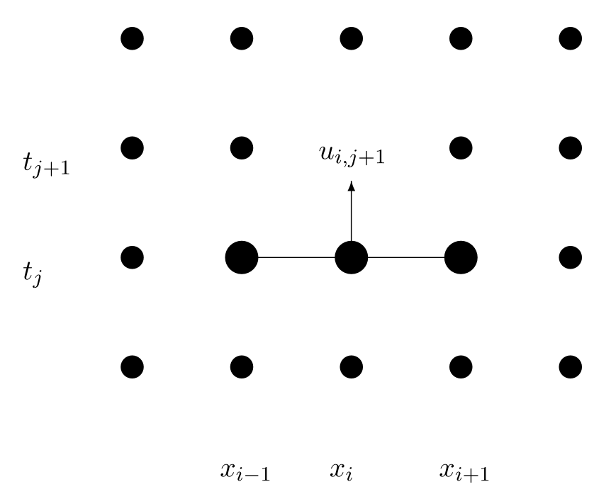
Notice that \(u_{i,j+1}\) depends on \(u_{i,j}\text{,}\) \(u_{i-1,j}\) and \(u_{i+1,j}\text{.}\) That is \(u\) at grid point \(i\) depends on its previous value and the values of its two nearest neighbors at the previous step (see Figure 4.6.1).

🔗

Schematic of information flow for the explicit method.🔗 — Figure 4.6.1. The value at grid point \((i,j+1)\) depends on its previous value and the previous values of its nearest neighbors.
🔗

🔗

Subsection 4.6.3 Initial Condition

To solve the partial differential equation (4.6.1) or (4.6.2) we need an initial condition. This represents the state of the system when we begin, i.e. the initial temperature distribution or initial concentration profile. This is represented by

\begin{equation*} u(x,0) = f(x)\text{.} \end{equation*}

To implement this in a program we let

\begin{equation*} u_{i,0}= f(x_{i})\text{.} \end{equation*}

🔗

Subsection 4.6.4 Boundary Conditions

To solve the partial differential equation ((4.6.1)) or ((4.6.2)) we also need boundary conditions. Just as in the previous section we will have to specify something about the ends of the domain, i.e. at \(x = 0\) and \(x = L\text{.}\) One possibility is fixed boundary conditions, which we can implement just as we did for the ODE boundary value problem.

🔗

A second possibility is called variable boundary conditions. This is represented by time-dependent functions,

\begin{equation*} u(0,t) = g_{1}(t) \quad\text{and}\quad u(L,t) = g_{2}(t)\text{.} \end{equation*}

In a heat problem, \(g_{1}\) and \(g_{2}\) would represent heating or cooling applied to the ends. These are easily implemented in a program by letting \(u_{0,j}= g_{1}(t_{j})\) and \(u_{m,j}= g_{2}(t_{j})\text{.}\)

🔗

Subsection 4.6.5 Implementation

The following program implements the explicit method. It incorporates variable boundary conditions at both ends. To run it you must define functions \(f\text{,}\) \(g_{1}\) and \(g_{2}\text{.}\) Notice that the main loop has only one line. The values of \(u\) are kept as a matrix. It is often convenient to define a matrix of the right dimension containing all zeros, and then fill in the calculated values as the program runs.

🔗

Program 4.6.2. myheat

🔗

function [t x u] = myheat(f,g1,g2,L,T,m,n,c)
    % function [t x u] = myheat(f,g1,g2,L,T,m,n,c)
    % solve u_t = c u_xx  for 0<=x<=L, 0<=t<=T
    %  BC:  u(0, t) = g1(t);  u(L,t) = g2(t)  
    %  IC:  u(x, 0) = f(x)
    % Inputs:  
    %    f -- function for IC
    %    g1,g2 -- functions for BC
    %    L -- length of rod
    %    T -- length of time interval
    %    m -- number of subintervals for x
    %    n -- number of subintervals for t
    %    c -- rate constant in equation
    % Outputs:
    %    t -- vector of time points
    %    x -- vector of x points
    %    u -- matrix of the solution, u(i,j)~=u(x(i),t(j))
    % Also plots.

    h = L/m;  k = T/n;          % set space and time step sizes
    r = c*k/h^2;  rr = 1 - 2*r;
    x = linspace(0,L,m+1);      % set space discretization
    t = linspace(0,T,n+1);      % set time discretization
    %Set up the matrix for u:
    u = zeros(m+1,n+1);
    % evaluate initial conditions
    u(:,1) = f(x);
    % evaluate boundary conditions
    u(1,:) = g1(t);  u(m+1,:) = g2(t);

    % find solution at remaining time steps
    for j = 1:n
        % explict method update at next time
        u(2:m,j+1) = r*u(1:m-1,j) + rr*u(2:m,j) + r*u(3:m+1,j);
    end

    % plot the results
    mesh(x,t,u')
end

Run the following program using \(L = 2\text{,}\) \(T=20\text{,}\) \(f(x) = .5 x\text{,}\) \(g_{1}(t) = 0\text{,}\) and \(g_{2}(t) = \cos(t)\text{.}\) You will find that simply g1 = @(t) 0 will not work, because it will only produce a single number \(0\text{.}\) Instead use g1 = @(t) 0*t, which will produce the needed vector of zeros.

🔗

Exercises 4.6.6 Exercises

1.

Run the program myheat.m (Program 4.6.2) with \(L = 2\pi\text{,}\) \(T=20\text{,}\) \(c = .5\text{,}\) \(g_{1}(t) = \sin(t)\text{,}\) \(g_{2}(t) =0\) and \(f(x) = -\sin(x/4)\text{.}\) Set \(m=20\) and experiment with \(n\text{.}\) Get a plot when the program is stable and one when it isn’t. Turn in the plots. Hint: The function \(g_{2}(t)\) will need to be input using the formula g2 = @(t) 0*t.

🔗

2.

Make a version of the program myheat.m (Program 4.6.2) that does not input \(n\) or \(T\) but instead has inputs:

%   k -- size of the time steps
%   temp -- keeps stepping in time until the maximum current 
%                 temperature in the bar is less than temp

For \(L = 2\pi\text{,}\) \(c = .01\text{,}\) \(g_{1}(t) = 0\text{,}\) \(g_{2}(t) = 10\text{,}\) \(f(x) = 100\) and \(m = 10\text{,}\) set \(k\) so that the method will be stable. Run it with temp = 20. (Hint: see your Exercise 4.2.5.2 as a model.) When does the temperature in the bar drop below 20? Turn in your program and the plot.

🔗

Prev Top Next