Nonlinear Systems - Newton’s Method

Section 2.6 Nonlinear Systems - Newton’s Method

Subsection 2.6.1 An Example

The LORAN (LOng RAnge Navigation) system calculates the position of a boat at sea using signals from fixed transmitters. From the time differences of the incoming signals, the boat obtains differences of distances to the transmitters. This leads to two equations each representing hyperbolas defined by the differences of distance of two points (foci). An example of such equations

E. Johnston, J. Mathews, Calculus, Addison-Wesley, 2001

are

\begin{equation} \begin{split}\frac{x^{2}}{186^{2}}- \frac{y^{2}}{300^{2} - 186^{2}}&= 1 \quad\text{and}\\ \frac{(y-500)^{2}}{279^{2}}- \frac{(x-300)^{2}}{500^{2} - 279^{2}}&= 1 \end{split}\text{.}\tag{2.6.1} \end{equation}

Solving two quadratic equations with two unknowns would require solving a 4 degree polynomial equation. We could do this by hand, but for a navigational system to work well, it must do the calculations automatically and numerically. We note that the Global Positioning System (GPS) works on similar principles and must do similar computations.

🔗

Subsection 2.6.2 Vector Notation

In general, we can usually find solutions to a system of equations when the number of unknowns matches the number of equations. Thus, we wish to find solutions to systems that have the form

\begin{equation} \begin{split}f_{1}(x_{1}, x_{2}, x_{3}, \ldots , x_{n})&= 0 \\ f_{2}(x_{1}, x_{2}, x_{3}, \ldots , x_{n})&= 0 \\ f_{3}(x_{1}, x_{2}, x_{3}, \ldots , x_{n})&= 0 \\ \vdots &\\ f_{n}(x_{1}, x_{2}, x_{3}, \ldots , x_{n})&= 0 \\\end{split}\text{.}\tag{2.6.2} \end{equation}

For convenience we can think of \((x_{1}, x_{2}, x_{3}, \ldots , x_{n})\) as a vector \(\xb\) and \((f_{1}, f_{2}, \ldots, f_{n})\) as a vector-valued function \(\fb\text{.}\) With this notation, we can write the system of equations (2.6.2) simply as

\begin{equation*} \fb(\xb) = \mathbf{0}\text{,} \end{equation*}

i.e. we wish to find a vector that makes the vector function equal to the zero vector.

🔗

As in Newton’s method for one variable, we need to start with an initial guess \(\xb_{0}\text{.}\) In theory, the more variables one has, the harder it is to find a good initial guess. In practice, this must be overcome by using physically reasonable assumptions about the possible values of a solution, i.e. take advantage of engineering knowledge of the problem.

🔗

Subsection 2.6.3 Linear Approximation for Vector Functions

In the single variable case, Newton’s method was derived by considering the linear approximation of the function \(f\) at the initial guess \(\xb_{0}\text{.}\) From Calculus, the following is the linear approximation of \(\fb\) at \(\xb_{0}\text{,}\) for vectors and vector-valued functions:

\begin{equation*} \fb(\xb) \approx \fb(\xb_{0}) + D\fb(\xb_{0}) (\xb - \xb_{0})\text{.} \end{equation*}

Here \(D\fb(\xb_{0})\) is an \(n \times n\) matrix whose entries are the various partial derivative of the components of \(\fb\text{,}\) evaluated at \(\xb_{0}\text{.}\) Specifically,

\begin{equation*} D\fb(\xb_{0}) = \left( \begin{array}{ccccc}\frac{\partial f_{1}}{\partial x_{1}}(\xb_0) & \frac{\partial f_{1}}{\partial x_{2}}(\xb_0) & \frac{\partial f_{1}}{\partial x_{3}}(\xb_0) & \ldots & \frac{\partial f_{1}}{\partial x_{n}}(\xb_0) \\ \frac{\partial f_{2}}{\partial x_{1}}(\xb_0) & \frac{\partial f_{2}}{\partial x_{2}}(\xb_0) & \frac{\partial f_{2}}{\partial x_{3}}(\xb_0) & \ldots & \frac{\partial f_{2}}{\partial x_{n}}(\xb_0) \\ \vdots & \vdots & \vdots & \ddots & \vdots \\ \frac{\partial f_{n}}{\partial x_{1}}(\xb_0) & \frac{\partial f_{n}}{\partial x_{2}}(\xb_0) & \frac{\partial f_{n}}{\partial x_{3}}(\xb_0) & \ldots & \frac{\partial f_{n}}{\partial x_{n}}(\xb_0)\end{array} \right)\text{.} \end{equation*}

🔗

Subsection 2.6.4 Newton’s Method

We wish to find \(\xb\) that makes \(\fb\) equal to the zero vectors, so let’s choose \(\xb_{1}\) so that

\begin{equation*} \fb(\xb_{0}) + D\fb(\xb_{0}) (\xb_{1} -\xb_{0}) = \mathbf{0}\text{.} \end{equation*}

Since \(D\fb(\xb_{0})\) is a square matrix, we can solve this equation by

\begin{equation*} \xb_{1} = \xb_{0} - (D\fb(\xb_{0}))^{-1}\fb(\xb_{0})\text{,} \end{equation*}

provided that the inverse exists. The formula is the vector equivalent of the Newton’s method formula we learned before. However, in practice we never use the inverse of a matrix for computations, so we cannot use this formula directly. Rather, we can do the following. First solve the equation

\begin{equation*} D\fb(\xb_{0}) \Delta \xb = -\fb(\xb_{0})\text{,} \end{equation*}

where we want to have

\begin{equation*} \Delta \xb = \xb_{1} - \xb_{0}\text{.} \end{equation*}

Since \(D\fb(\xb_{0})\) is a known matrix and \(-\fb(\xb_{0})\) is a known vector, this equation is just a system of linear equations, which can be solved efficiently and accurately. Once we have the solution vector \(\Delta \xb\text{,}\) we can obtain our improved estimate \(\xb_{1}\) by

\begin{equation*} \xb_{1} = \xb_{0} + \Delta \xb\text{.} \end{equation*}

🔗

For subsequent steps, we have the following process:

Solve \(D\fb(\xb_{i}) \Delta \xb = -\fb(\xb_{i})\) for \(\Delta \xb\text{.}\)
🔗

🔗
Let \(\xb_{i+1}= \xb_{i} + \Delta \xb\)
🔗

🔗

🔗

Subsection 2.6.5 An Experiment

We will solve the following set of equations:

\begin{equation*} \begin{split}x^{3} + y&= 1 \\ y^{3} - x&= -1\end{split}\text{.} \end{equation*}

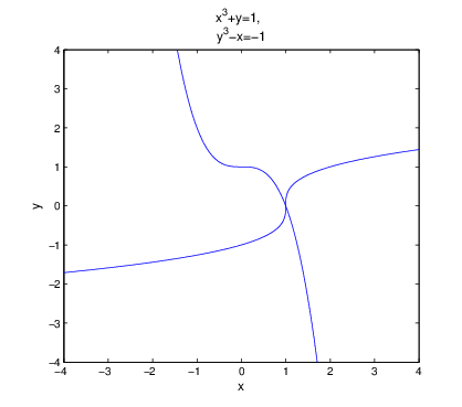
You can easily check that \((x,y) = (1,0)\) is a solution of this system. By graphing both of the equations you can also see that \((1,0)\) is the only solution Figure 2.6.1.

🔗

Solution curves of two nonlinear equations.🔗 — Figure 2.6.1. Graphs of the equations \(x^{3} + y = 1\) and \(y^{3} - x = -1\text{.}\) There is one and only one intersection; at \((x,y) = (1,0)\text{.}\)
🔗

We can put these equations into vector-function form (2.6.2) by letting \(x_{1} = x\text{,}\) \(x_{2} = y\) and

\begin{equation*} \begin{split}f_{1}(x_{1},x_{2})&= x_{1}^{3} + x_{2} - 1 \\ f_{2}(x_{1},x_{2})&= x_{2}^{3} - x_{1} + 1\end{split}\text{,} \end{equation*}

or, equivalently,

\begin{equation*} \fb(\xb) = \left(\begin{array}{c}x_1^3 + x_2 - 1 \\ x_2^3 - x_1 + 1\end{array} \right)\text{.} \end{equation*}

🔗

The partial derivatives are

\begin{equation} \frac{\partial f_{1}}{\partial x_{1}}= 3 x_{1}^{2}, \quad \frac{\partial f_{1}}{\partial x_{2}}= 1, \quad \frac{\partial f_{2}}{\partial x_{1}}= -1, \quad\text{and}\quad \frac{\partial f_{2}}{\partial x_{2}}= 3 x_{2}^{2}\text{.}\tag{2.6.3} \end{equation}

Thus,

\begin{equation} D \mathbf{f}= \left(\begin{array}{cc}3x_1^2 & 1 \\ -1 & 3x_2^2\end{array} \right)\text{.}\tag{2.6.4} \end{equation}

Now that we have the equations in vector-function form, we can write the following script program:

format long; 
f = @(x)[ x(1)^3+x(2)-1 ; x(2)^3-x(1)+1 ] 
x = [.5;.5] 
x = fsolve(f,x)

Save this program as myfsolve.m and run it. You will see that the internal MATLAB solving command fsolve approximates the solution, but only to about 7 decimal places. While that would be close enough for most applications, one would expect that we could do better on such a simple problem.

🔗

Next we will implement Newton’s method for this problem. Modify your myfsolve program to:

% mymultnewton - solve an example nonlinear system
format long;
n=8  % set some number of iterations, may need adjusting
f = @(x)[x(1)^3+x(2)-1 ; x(2)^3-x(1)+1] % the vector function
% the matrix of partial derivatives
Df = @(x)[3*x(1)^2,  1 ; -1,  3*x(2)^2] 
x = [.5;.5]             % starting guess
for i = 1:n
      Dx = -Df(x)\f(x); % solve for increment
      x = x + Dx        % add on to get new guess
      f(x)              % see if f(x) is really zero
end

Save and run this program (as mymultnewton) and you will see that it finds the root exactly (to machine precision) in only 6 iterations. Why is this simple program able to do better than MATLAB’s built-in program?

🔗

Exercises 2.6.6 Exercises

1.

Put the LORAN equations (2.6.1) into the function form (2.6.2).
🔗

🔗
Calculate (by hand) the partial derivatives of \(\mathbf{f}\) and construct the matrix \(D\fb\) (see (2.6.3) and (2.6.4)).
🔗

🔗
Adapt the mymultnewton program to find a solution for these equations. By trying different starting vectors, find at least three different solutions. (There are actually four solutions.)
🔗

🔗
Think of at least one way that the navigational system could determine the correct solution.
🔗

🔗

🔗

Prev Top Next