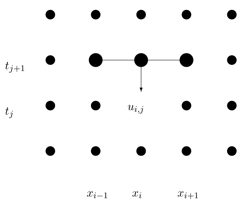
By approximating \(u_{xx}\) and \(u_{t}\) at \(t_{j+1}\) rather than \(t_{j}\text{,}\) and using a backwards difference for \(u_{t}\text{,}\) the equation \(u_{t} = c u_{xx}\) is approximated by
Now we have \(\ub_{j}\) given in terms of \(\ub_{j+1}\text{.}\) This seems like a problem, since \(\ub_{j+1}\) is the solution at a later time than \(\ub_{j}\text{,}\) so we could never know \(\ub_{j+1}\) before we knew \(\ub_{j}\text{.}\) However, the relationship between \(\ub_{j+1}\) and \(\ub_{j}\) is linear. Using matrix notation, we have
\begin{equation*}
\ub_{j} = B \ub_{j+1}- r \bb_{j+1}\text{,}
\end{equation*}
where \(\bb_{j+1}\) represents the boundary conditions. Thus to find \(\ub_{j+1}\) from \(\ub_{j}\text{,}\) we need only solve the linear system
\begin{equation}
B \ub_{j+1}= \ub_{j} + r \bb_{j+1}\,\text{,}\tag{4.8.2}
\end{equation}
(This is an example of how a sparse matrix occurs in applications.) Using this scheme is called the implicit method since \(\ub_{j+1}\) is defined implicitly. Since we have to solve a linear system at each step, the implicit method requires more work per step than the explicit method.
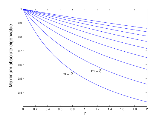
Since we are solving (4.8.2), the most important quantity is the maximum absolute eigenvalue of \(B^{-1}\text{,}\) which is 1 divided by the smallest eigenvalue of \(B\text{.}\)Figure 4.8.2 shows the maximum absolute eigenvalues of \(B^{-1}\) as a function of \(r\) for various size matrices.
Figure4.8.2.Maximum absolute eigenvalue as a function of \(r\) for the matrix \(B^{-1}\) from the implicit method for the heat equation calculated for matrices \(B\) of sizes \(m = 2 \ldots 10\text{.}\) Whenever the maximum absolute eigenvalue is less than 1 the method is stable, i.e. it is always stable.
Notice that this absolute maximum is always less than \(1\text{.}\) Thus errors are always diminished over time and so this method is always stable. For the same reason it is also always as accurate as the individual steps.
Both this implicit method and the explicit method in the previous section make \(O(h^{2})\) error in approximating \(u_{xx}\) and \(O(k)\) error in approximating \(u_{t}\text{,}\) so they have total error \(O(h^{2}+k)\text{.}\) Thus although the stability condition allows the implicit method to use arbitrarily large \(k\text{,}\) to maintain accuracy we still need \(k\sim h^{2}\text{.}\)
Now that we have two different methods for solving parabolic equation, it is natural to ask, “can we improve by taking an average of the two methods?” The answer is yes.
We implement a weighted average of the two methods by considering an average of the approximations of \(u_{xx}\) at \(j\) and \(j+1\text{.}\) This leads to the equations
In this equation \(\ub_{j}\) and \(\bb_{j+1}\) are known, \(A \ub_{j}\) can be calculated directly, and then the equation is solved for \(\ub_{j+1}\text{.}\)
If we choose \(\lambda=1/2\text{,}\) then we are in effect doing a central difference for \(u_{t}\text{,}\) which has error \(O(k^{2})\text{.}\) Our total error is then \(O(h^{2}+k^{2})\text{.}\) With a bit of work, we can show that the method is always stable, and so we can use \(k\sim h\) without a problem.
To get optimal accuracy with a weighted average, it is always necessary to use the right weights. For the Crank-Nicholson method with a given \(r\text{,}\) we need to choose
This choice will make the method have truncation error of order \(O(h^{4} + k^{2})\text{,}\) which is really good considering that the implicit and explicit methods each have truncation errors of order \(O(h^{2} + k)\text{.}\) Surprisingly, we can do even better if we also require
\begin{equation*}
r = \frac{\sqrt{5}}{10}\approx 0.22361\text{,}
\end{equation*}
To appreciate the implications, suppose that we need to solve a problem with 4 significant digits. If we use the explicit or implicit method alone then we will need \(h^{2} \approx k \approx 10^{-4}\text{.}\) If \(L=1\) and \(T\approx 1\text{,}\) then we need \(m \approx 100\) and \(n \approx 10,000\text{.}\) Thus we would have a total of \(1,000,000\) grid points, almost all in the interior. This is a lot.
Next suppose we solve the same problem using the optimal Crank-Nicholson method. We would need \(h^{6} \approx 10^{-4}\) which would require us to take \(m \approx 4.64\text{,}\) so we would take \(m = 5\) and have \(h=1/5\text{.}\) For \(k\) we need \(k = (\sqrt{5}/10) h^{2}/c\text{.}\) If \(c=1\text{,}\) this gives \(k = \sqrt{5}/250\approx 0.0089442\) so we would need \(n\approx 112\) to get \(T\approx 1\text{.}\) This gives us a total of \(560\) interior grid points, or, a factor of \(1785\) fewer than the explicit or implicit method alone.
Modify the program myexpmatrix.m (Program 4.7.2) into a function program myimpmatrix.m that produces the matrix \(B\) in (4.8.3) for given inputs \(m\) and \(r\text{.}\) Modify your script from Exercise 4.7.3.2 to use \(B^{-1}\) and to plot for \(r\in[0,2]\text{;}\) keep \(m = 4\text{.}\) It should produce a graph similar to that in Figure 4.8.2 for \(m = 4\text{.}\) Turn in the programs and the plot.
(Hints: Delete g1 and g2 from the program since they are always zero. Call \(B\) using myimpmatrix before the loop and solve \(B \ub_{j+1}= \ub_{j}\) inside the loop.)
Run the program with \(L=5\text{,}\)\(T=50\text{,}\)\(c=.1\) and \(f(x) = \sin( \pi x/5)\) and at least 10 pairs of values of \(m\) and \(n\text{.}\) Turn in the program and a list of the \(m,n\) you tried and whether the simulation was stable or unstable. Are you convinced that it is always stable?