Finite Elements

Section 4.11 Finite Elements

Subsection 4.11.1 Triangulating a Region

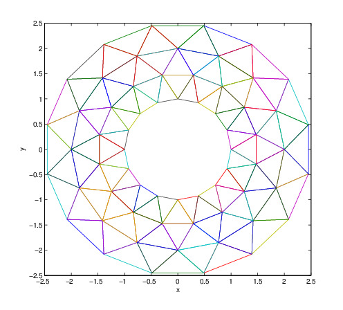
A disadvantage of finite difference methods is that they require a very regular grid, and thus a very regular region, either rectangular or a regular part of a rectangle. Finite elements is a method that works for any shape region because it is not built on a grid, but on triangulation of the region, i.e. cutting the region up into triangles as we did in a previous section. The following figure shows a triangularization of a region.

🔗

Plot of a washer made of triangles.🔗 — Figure 4.11.1. An annular region with a triangulation. Notice that the nodes and triangles are very evenly spaced.
🔗

This figure was produced by the script program mywasher.m (Program A.2.8). Notice that the nodes are evenly distributed. This is good for the finite element process where we will use it.

🔗

Open the program mywasher.m (Program A.2.8). This program defines a triangulation by defining the vertices in a matrix V in which each row contains the \(x\) and \(y\) coordinates of a vertex. Notice that we list the interior nodes first, then the boundary nodes.

🔗

Triangles are defined in the matrix T. Each row of T has three integer numbers indicating the indices of the nodes that form a triangle. For instance the first row is 43 42 25, so \(T_{1}\) is the triangle with vertices \(\vb_{43}\text{,}\) \(\vb_{42}\) and \(\vb_{25}\text{.}\) The matrix \(T\) in this case was produced by the MATLAB command delaunay. The command produced more triangles than desired and the unwanted ones were deleted.

🔗

A three dimensional plot of the region and triangles is produced by having the last line be trimesh(T,x,y,z).

🔗

Subsection 4.11.2 What is a finite element?

The finite element method is a mathematically complicated process. However, a finite element is actually a very simple object. To each node \(\vb_{j}\) we associate a function \(\Phi_{j}\) that has the properties \(\Phi_{j}(\vb_{j})=1\) and \(\Phi_{j}(\vb_{i})=0\) for \(i\not=j\text{.}\) Between nodes, \(\Phi_{j}\) is a linear function. This function is the finite element. (There are fancier types of finite elements that we will not discuss.)

🔗

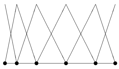
If we consider one dimension, then a triangulation is just a subdivision into subintervals. In Figure 4.11.2 we show an uneven subdivision of an interval and the finite elements corresponding to each node.

🔗

Schematic of 1D finite elements.🔗 — Figure 4.11.2. The finite elements for the “triangulation” of a one dimensional object.
🔗

In two dimensions, \(\Phi_{j}\) is composed of triangular piece of planes. Thus \(\Phi_{j}\) is a function whose graph is a pyramid with its peak over node \(\vb_{j}\text{.}\) For an example, try:

>> mywasher
>> z = 0*z;
>> z(1) =1
>> trimesh(T,x,y,z)

🔗

Subsection 4.11.3 What is a finite element solution?

A finite element (approximate) solution is a linear combination of the elements:

\begin{equation*} U(\xb) = \sum_{j=1}^{n} C_{j} \Phi_{j}(\xb)\text{.} \end{equation*}

Thus finding a finite element solution amounts to finding the best values for the constants \(\{ C_{j} \}_{j=1}^{n}\text{.}\)

🔗

In the program mywasher.m (Program A.2.8), the vector z contains the node values \(C_{j}\text{.}\) These values give the height at each node in the graph. For instance if we set all equal to \(0\) except one equal to \(1\text{,}\) then the function is a finite element. Do this for one boundary node, then for one interior node.

🔗

Notice that a sum of linear functions is a linear function. Thus the solution using linear elements is a piecewise linear function. Also notice that if we denote the \(j\)-th vertex by \(\vb_{j}\text{,}\) then

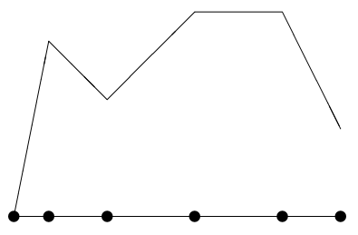
\begin{equation*} U(\vb_{j}) = C_{j}\text{.} \end{equation*}

Thus we see that the constants \(C_{j}\) are just the values at the nodes.

🔗

Take the one-dimensional case. Since we know that the solution is linear on each subinterval, knowing the values at the endpoints of the subintervals, i.e. the nodes, gives us complete knowledge of the solution. Figure 4.11.3 could be a finite element solution since it is piecewise linear.

🔗

Schematic of 1D finite element solution.🔗 — Figure 4.11.3. A possible finite element solution for a one dimensional object. Values are assigned at each node and a linear interpolant is used in between.
🔗

In the two-dimensional case, the solution is linear on each triangle, and so again, if we know the values \(\{C_{j}\}_{j=1}^{n}\) at the nodes then we know everything.

🔗

Subsection 4.11.4 Experiment with finite elements

By changing the values in z in the program we can produce different three dimensional shapes based on the triangles. The point then of a finite element solution is to find the values at the nodes that best approximate the true solution. This task can be subdivided into two parts: (1) assigning the values at the boundary nodes and (2) assigning the values at the interior nodes.

🔗

Subsection 4.11.5 Values at boundary nodes

Once a triangulation and a set of finite elements is set up, the next step is to incorporate the boundary conditions of the problem. Suppose that we have fixed boundary conditions, i.e. of the form

\begin{equation*} u(\xb) = g(\xb) \quad \text{for}\quad \xb \in \partial D\text{,} \end{equation*}

where \(D\) is the object (domain) and \(\partial D\) is its boundary. Then the boundary condition directly determines the values on the boundary nodes.

🔗

In particular, suppose that \(\vb_{\ell}\) is a boundary node. Since \(\Phi_{\ell}(\vb_{\ell}) = 1\) and all the other elements are zero at node \(\vb_{\ell}\text{,}\) then to make

\begin{equation*} U(\vb_{\ell}) = \sum_{j=1}^{n} C_{j} \Phi_{j}(\vb_{\ell}) = g(\vb_{\ell})\text{,} \end{equation*}

we must choose

\begin{equation*} C_{\ell} = g(\vb_{\ell})\text{.} \end{equation*}

Thus the constants \(C_{j}\) for the boundary nodes are set at exactly the value of the boundary condition at the nodes.

🔗

Thus, if there are \(m\) interior nodes, then

\begin{equation*} C_{j} = g(\vb_{j}), \qquad \text{for all}\quad m+1 \le j \le n\text{.} \end{equation*}

🔗

In the program mywasher.m (Program A.2.8), the first 32 vertices correspond to interior nodes and the last 32 correspond to boundary nodes. By setting the last 32 values of z, we achieve the boundary conditions. We could do this by adding the following commands to the program:

z(33:64) = .5;

or more elaborately we might use functions:

z(33:48) = x(33:48).^2 - .5*y(33:48).^2; 
z(49:64) = .2*cos(y(49:64));

🔗

Exercises 4.11.6 Exercises

1.

Generate an interesting or useful 2-d object and a well-distributed triangulation of it. Make it have at least 2 interior nodes and have it list the interior nodes before the boundary nodes.

Plot the region.
🔗

🔗
Plot one interior finite element.
🔗

🔗
Plot one boundary finite element.
🔗

🔗
Assign values to the boundary using a function (or functions) and plot the region with the boundary values.
🔗

🔗

Turn in your code and the four plots.

🔗

Prev Top Next