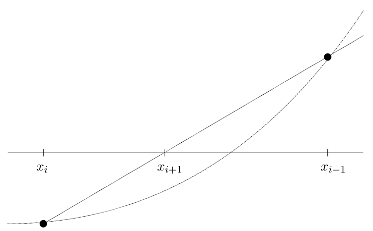
In this section we introduce two additional methods to find numerical solutions of the equation \(f(x) = 0\text{.}\) Both of these methods are based on approximating the function by secant lines just as Newton’s method was based on approximating the function by tangent lines.
The secant method requires two initial approximations \(x_{0}\) and \(x_{1}\text{,}\) preferably both reasonably close to the solution \(x^{*}\text{.}\) From \(x_{0}\) and \(x_{1}\) we can determine that the points \((x_{0},y_{0}=f(x_{0}))\) and \((x_{1},y_{1}=f(x_{1}))\) both lie on the graph of \(f\text{.}\) Connecting these points gives the (secant) line
Since we want \(f(x)=0\text{,}\) we set \(y=0\text{,}\) solve for \(x\text{,}\) and use that as our next approximation. Repeating this process gives us the iteration
For example, suppose \(f(x) = x^{4}-5\text{,}\) which has a solution \(x^{*} = \sqrt[4]{5}\approx 1.5\text{.}\) Choose \(x_{0}=1\) and \(x_{1} = 2\) as initial approximations. Next we have that \(y_{0} = f(1) = -4\) and \(y_{1} = f(2) = 11\text{.}\) We may then calculate \(x_{2}\) from the formula (1.6.1):
Pluggin \(x_{2} = 19/15\) into \(f(x)\) we obtain \(y_{2} = f(19/15) \approx -2.425758...\text{.}\) In the next step we would use \(x_{1} = 2\) and \(x_{2} = 19/15\) in the formula (1.6.1) to find \(x_{3}\) and so on.
Below is a program for the secant method. Notice that it requires two input guesses \(x_{0}\) and \(x_{1}\text{,}\) but it does not require the derivative to be input.
Program1.6.2.mysecant
function x = mysecant(f,x0,x1,n)
    % Solves f(x) = 0 by doing n steps of the secant method
    %   starting with x0 and x1.
    % Inputs: f -- the function
    %         x0 -- starting guess, a number
    %         x1 -- second starting guess
    %         n -- the number of steps to do
    % Output: x -- the approximate solution
    y0 = f(x0);
    y1 = f(x1);
    for i = 1:n               % Do n times
        x = x1 - (x1-x0)*y1/(y1-y0)    % secant formula.
        y=f(x)           % y value at the new approximate solution.
        % Move numbers to get ready for the next step
        x0=x1;
        y0=y1;
        x1=x;
        y1=y;
    end
end
The Regula Falsi method is a combination of the secant method and bisection method. As in the bisection method, we have to start with two approximations \(a\) and \(b\) for which \(f(a)\) and \(f(b)\) have different signs. As in the secant method, we follow the secant line to get a new approximation, which gives a formula similar to (1.6.1),
\begin{equation*}
x = b - \frac{b - a}{f(b) - f(a)}f(b) \,.
\end{equation*}
Then, as in the bisection method, we check the sign of \(f(x)\text{;}\) if it is the same as the sign of \(f(a)\) then \(x\) becomes the new \(a\) and otherwise let \(x\) becomes the new \(b\text{.}\) Note that in general either \(a\rightarrow x^{*}\) or \(b\rightarrow x^{*}\) but not both, so \(b-a \not\rightarrow 0\text{.}\) For example, for the function in Figure 1.6.1, \(a\rightarrow x^{*}\) but \(b\) would never move.
If we can begin with a good choice \(x_{0}\text{,}\) then Newton’s method will converge to \(x^{*}\) rapidly. The secant method is a little slower than Newton’s method and the Regula Falsi method is slightly slower than that. However, both are still much faster than the bisection method.
If we do not have a good starting point or interval, then the secant method, just like Newton’s method, can fail altogether. The Regula Falsi method, just like the bisection method, always works because it keeps the solution inside a definite interval.
Although Newton’s method converges faster than any other method, there are contexts when it is not convenient, or even impossible. One obvious situation is when it is difficult to calculate a formula for \(f'(x)\) even though one knows the formula for \(f(x)\text{.}\) This is often the case when \(f(x)\) is not defined explicitly, but implicitly. There are other situations, which are very common in engineering and science, where even a formula for \(f(x)\) is not known. This happens when \(f(x)\) is the result of experiment or simulation rather than a formula. In such situations, the secant method is usually the best choice.
Perform 3 iterations of the secant method on the function \(f(x) = x^{2}-5\text{,}\) with starting points \(x_{-1}= 1\) and \(x_{0}=3\text{.}\) (By hand, but use a calculator.) Calculate the errors and percentage errors of \(x_{1}\text{,}\)\(x_{2}\text{,}\) and \(x_{3}\text{.}\) Compare the errors with those in Exercise 1.3.5.2 and Exercise 1.5.4.2
Create and graph the function g = @(x) log(x)+x.^2. In the plot window, use the Tools menu to zoom in on the root (there is only one) to 2 decimal places. From this determine good starting points a0 and b0 and use the program mysecant.m (Program 1.6.2) to approximate the root \(x^{*}\) to 15 decimal places. Turn in your zoomed-in plot and your approximation.
Modify the program mysecant.m (Program 1.6.2) to iterate until the absolute value of the residual is less than a given tolerance. (Let tol be an input instead of n.) Modify the comments appropriately. Test program on the two functions in the exercises above with tol\(= 10^{-10}\text{.}\) Turn in the results and the program.