
Section 4.7 Solution Instability for the Explicit Method

As we saw in experiments using myheat.m (Program 4.6.2), the solution can become unbounded unless the time steps are small. In this section we consider why.

Subsection 4.7.1 Writing the Difference Equations in Matrix Form

If we use the boundary conditions \(u(0) = u(L) = 0\) then the explicit method of the previous section has the form
\begin{equation*} u_{i,j+1}= r u_{i-1,j}+ (1 - 2r) u_{i,j}+ r u_{i+1,j}\quad\text{for}\quad 1 \le i \le m-1\quad\text{and}\quad 0 \le j \le n-1 \text{,} \end{equation*}
where \(u_{0,j}= 0\) and \(u_{m,j}=0\text{.}\) This is equivalent to the matrix equation
\begin{equation} \ub_{j+1}= A \ub_{j}\text{,}\tag{4.7.1} \end{equation}
where \(\ub_{j}\) is the column vector \((u_{1,j}, u_{2,j}, \ldots, u_{m,j})'\) representing the state at the \(j\)th time step and \(A\) is the matrix
\begin{equation} A = \left( \begin{array}{ccccc}1-2r & r & 0 & \cdots & 0 \\ r & 1-2r & r & \ddots & \vdots \\ 0 & \ddots & \ddots & \ddots & 0 \\ \vdots & \ddots & r & 1-2r & r \\ 0 & \cdots & 0 & r & 1-2r\end{array} \right)\text{.}\tag{4.7.2} \end{equation}
Unfortunately, this matrix can have a property which is very bad in this context. Namely, it can cause exponential growth of error unless \(r\) is small. To see how this happens, suppose that \(\Ub_{j}\) is the vector of correct values of \(u\) at time step \(t_{j}\) and \(\Eb_{j}\) is the error of the approximation \(\ub_{j}\text{,}\) then
\begin{equation*} \ub_{j} = \Ub_{j} + \Eb_{j}\text{.} \end{equation*}
From (4.7.1), the approximation at the next time step will be
\begin{equation*} \ub_{j+1}= A \Ub_{j} + A \Eb_{j}\text{,} \end{equation*}
and if we continue for \(k\) steps,
\begin{equation*} \ub_{j+k}= A^{k} \Ub_{j} + A^{k} \Eb_{j}\text{.} \end{equation*}
The problem with this is the term \(A^{k} \Eb_{j}\text{.}\) This term is exactly what we would do in the power method for finding the eigenvalue of \(A\) with the largest absolute value. If the matrix \(A\) has eigenvalues with absolute value greater than \(1\text{,}\) then this term will grow exponentially. Figure 4.7.1 shows the largest absolute value of an eigenvalue of \(A\) as a function of the parameter \(r\) for various sizes of the matrix \(A\text{.}\) As you can see, for \(r> 1/2\) the largest absolute eigenvalue grows rapidly for any \(m\) and quickly becomes greater than \(1\text{.}\)
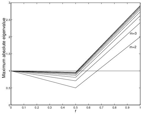
Plot of spectra for the explicit method.🔗
Figure 4.7.1. Maximum absolute eigenvalue as a function of \(r\) for the matrix \(A\) from the explicit method for the heat equation calculated for matrices \(A\) of sizes \(m = 2 \ldots 10\text{.}\) Whenever the maximum absolute eigenvalue is greater than 1 the method is unstable, i.e. errors grow exponentially with each step. When using the explicit method \(r < 1/2\) is a safe choice.

Subsection 4.7.2 Consequences

Recall that \(r = ck/h^{2}\text{.}\) Since this must be less than 1/2, we have
\begin{equation*} k < \frac{h^{2}}{2c}\text{.} \end{equation*}
The first consequence is obvious: \(k\) must be relatively small.The second is that \(h\) cannot be too small. Since \(h^{2}\) appears in the formula, making \(h\) small would force \(k\) to be extremely small!A third consequence is that we have a converse of this analysis. Suppose \(r < .5\text{.}\) Then all the eigenvalues will be less than one. Recall that the error terms satisfy
\begin{equation*} \ub_{j+k}= A^{k} \Ub_{j} + A^{k} \Eb_{j}\text{.} \end{equation*}
If all the eigenvalues of \(A\) are less than \(1\) in absolute value then \(A^{k} \Eb_{j}\) grows smaller and smaller as \(k\) increases. This is really good. Rather than building up, the effect of any error diminishes as time passes! From this we arrive at the following principle: If the explicit numerical solution for a parabolic equation does not blow up, then errors from previous steps fade away!
Finally, we note that if we have non-zero boundary conditions then instead of equation ((4.7.1)) we have
\begin{equation*} \ub_{j+1}= A \ub_{j} + r \bb_{j}\text{,} \end{equation*}
where the first and last entries of \(\bb_{j}\) contain the boundary conditions and all the other entries are zero. In this case the errors behave just as before, if \(r> 1/2\) then the errors grow and if \(r<1/2\) the errors fade away.
We can write a function program myexpmatrix.m that produces the matrix \(A\) in (4.7.2), for given inputs \(m\) and \(r\text{.}\) Without using loops we can use the diag command to set up the matrix:
Program 4.7.2. myexpmatrix
function A = myexpmatrix(m,r)
    % produces the matrix for the explicit method for a parabolic equation
    % Inputs: m -- the size of the matrix
    %         r -- the main parameter, ck/h^2
    % Output: A -- an m by m matrix
    u = (1-2*r)*ones(m,1);  % make a vector for the main diagonal
    v = r*ones(m-1,1);    % make a vector for the upper and lower diagonals
    A = diag(u) + diag(v,1) + diag(v,-1);  % assemble
end
Test this using \(m=6\) and \(r=.4, .6\text{.}\) Check the eigenvalues and eigenvectors of the resulting matirices:
>> A = myexpmatrix(6,.6)
>> [v e] = eig(A)
What is the “mode” represented by the eigenvector with the largest absolute eigenvalue? How is that reflected in the unstable solutions?

Exercises 4.7.3 Exercises

1.

Let \(L=\pi\text{,}\) \(T = 20\text{,}\) \(f(x) = .1\sin(x)\text{,}\) \(g_{1}(t) = 0\text{,}\) \(g_{2}(t) = 0\text{,}\) \(c = .5\text{,}\) and \(m = 20\text{,}\) as used in the program myheat.m (Program 4.6.2). What value of \(n\) corresponds to \(r = 1/2\text{?}\) Try different \(n\) in myheat.m to find precisely when the method works and when it fails. Is \(r = 1/2\) the boundary between failure and success? Hand in a plot of the last success and the first failure. Include the values of \(n\) and \(r\) in each.

2.

Write a well-commented MATLAB script program that produces the graph in Figure 4.7.1 for \(m = 4\text{.}\) Your program should:

