Integration: Midpoint and Simpson’s Rules

Section 3.4 Integration: Midpoint and Simpson’s Rules

Subsection 3.4.1 Midpoint rule

If we use the endpoints of the subintervals to approximate the integral, we run the risk that the values at the endpoints do not accurately represent the average value of the function on the subinterval. A point which is much more likely to be close to the average would be the midpoint of each subinterval. Using the midpoint in the sum is called the midpoint rule. On the \(i\)-th interval \([x_{i-1},x_{i}]\) we will call the midpoint \(\bar{x}_{i}\text{,}\) i.e.

\begin{equation*} \bar{x}_{i} = \frac{ x_{i-1}+ x_{i}}{2}\text{.} \end{equation*}

If \(\Delta x_{i} = x_{i} - x_{i-1}\) is the length of each interval, then using midpoints to approximate the integral would give the formula

\begin{equation*} M_{n} = \sum_{i=1}^{n} f(\bar{x}_{i}) \Delta x_{i}\text{.} \end{equation*}

For even spacing, \(\Delta x_{i} = h = (b-a)/n\text{,}\) and the formula is

\begin{equation} M_{n} = h \, \sum_{i=1}^{n}f(\bar{x}_{i}) = h \, (\hat{y}_{1} + \hat{y}_{2} + \ldots + \hat{y}_{n})\text{,}\tag{3.4.1} \end{equation}

where we define \(\hat{y}_{i} = f(\bar{x}_{i})\text{.}\)

🔗

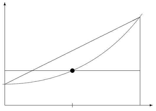
While the midpoint method is obviously better than \(L_{n}\) or \(R_{n}\text{,}\) it is not obvious that it is actually better than the trapezoid method \(T_{n}\text{,}\) but it is.

🔗

Subsection 3.4.2 Simpson’s rule

Consider Figure 3.4.1.

🔗

Diagram with the trapezoid rule and midpoint rule.🔗 — Figure 3.4.1. Comparing the trapezoid and midpoint method on a single subinterval. The function is concave up, in which case \(T_{n}\) is too high, while \(M_{n}\) is too low.
🔗

If \(f\) is not linear on a subinterval, then it can be seen that the errors for the midpoint and trapezoid rules behave in a very predictable way, they have opposite sign. For example, if the function is concave up then \(T_{n}\) will be too high, while \(M_{n}\) will be too low. Thus it makes sense that a better estimate would be to average \(T_{n}\) and \(M_{n}\text{.}\) However, in this case we can do better than a simple average. The error will be minimized if we use a weighted average. To find the proper weight we take advantage of the fact that for a quadratic function the errors \(EM_{n}\) and \(ET_{n}\) are exactly related by

\begin{equation*} |EM_{n}| = \frac{1}{2}|ET_{n}|\text{.} \end{equation*}

Thus we take the following weighted average of the two, which is called Simpson’s rule:

\begin{equation*} S_{2n}= \frac{2}{3}M_{n} + \frac{1}{3}T_{n}\text{.} \end{equation*}

If we use this weighting on a quadratic function the two errors will exactly cancel.

🔗

Notice that we write the subscript as \(2n\text{.}\) That is because we usually think of \(2n\) subintervals in the approximation; the \(n\) subintervals of the trapezoid are further subdivided by the midpoints. We can then number all the points using integers. If we number them this way we notice that the number of subintervals must be an even number.

🔗

The formula for Simpson’s rule if the subintervals are evenly spaced is the following (with \(n\) intervals, where \(n\) is even):

\begin{equation*} S_{n} = \frac{h}{3}\left( f(x_{0}) + 4f(x_{1}) + 2f(x_{2}) + 4f(x_{3}) + \ldots + 2f(x_{n-2}) + 4f(x_{n-1}) + f(x_{n}) \right)\text{.} \end{equation*}

🔗

Note that if we are presented with data \(\{x_{i},y_{i}\}\) where the \(x_{i}\) points are evenly spaced with \(x_{i+1}- x_{i} = \Delta x\text{,}\) it is easy to apply Simpson’s method:

\begin{equation} S_{n} = \frac{h}{3}\left( y_{0} + 4 y_{1} + 2 y_{2} + 4 y_{3} + \ldots + 2 y_{n-2}+ 4 y_{n-1}+ y_{n} \right).\tag{3.4.2} \end{equation}

Notice the pattern of the coefficients. The following program will produce these coefficients for \(n\) intervals, if \(n\) is an even number. Try it for \(n = 6,7,100\text{.}\)

Program 3.4.2. mysimpweights

🔗

function w = mysimpweights(n)
    % Computes the weights for Simpson's rule
    % Input:  n -- the number of intervals, must be even
    % Output: w -- a (column) vector with the weights, length n+1
    if rem(n,2) ~= 0
        error('n must be even for Simpsons rule')
    end
    w = 2*ones(n+1,1); % column vector, starts all 2's
    w(1) = 1; w(n+1) = 1; % set ends to 1's
    w(2:2:n)=4; % set even # entries to 4.
end

🔗

Simpson’s rule is incredibly accurate. We will consider just how accurate in the next section. The one drawback is that the points used must either be evenly spaced, or at least the odd number points must lie exactly at the midpoint between the even numbered points. In applications where you can choose the spacing, this is not a problem. In applications such as experimental or simulated data, you might not have control over the spacing and then you cannot use Simpson’s rule.

🔗

Subsection 3.4.3 Error bounds

The trapezoid, midpoint, and Simpson’s rules are all approximations. As with any approximation, before you can safely use it, you must know how good (or bad) the approximation might be. For these methods there are formulas that give upper bounds on the error. In other words, the worst case errors for the methods. These bounds are given by the following statements:

🔗

Suppose \(f''\) is continuous on \([a,b]\text{.}\) Let \(K_{2} = \max_{x \in [a,b]}|f''(x)|\text{.}\) Then the errors \(ET_{n}\) and \(EM_{n}\) of the Trapezoid and Midpoint rules, respectively, applied to \(\int_{a}^{b} f \, dx\) satisfy

\begin{equation*} |ET_{n}|\le K_{2} \frac{b-a}{12}h^{2} \end{equation*}

and

\begin{equation*} |EM_{n}| \le K_{2}\frac{b-a}{24}h^{2}\text{.} \end{equation*}

🔗

🔗
Suppose \(f^{(4)}\) is continuous on \([a,b]\text{.}\) Let \(K_{4} = \max_{x \in [a,b]}|f^{(4)}(x)|\text{.}\) Then the error \(ES_{n}\) of Simpson’s rule applied to \(\int_{a}^{b} f \, dx\) satisfies

\begin{equation*} |ES_{n}| \le K_{4}\frac{b-a}{180}h^{4}. \end{equation*}

🔗

🔗

In practice \(K_{2}\) and \(K_{4}\) are themselves approximated from the values of \(f\) at the evaluation points.

🔗

The most important thing in these error bounds is the dependence on \(h\text{.}\) To emphasize this dependence, we sometimes use the order notation \(O(\;)\text{.}\) The trapezoid and midpoint method errors are \(O(h^{2})\text{,}\) so the methods have order 2. The Simpson’s rule error is \(O(h^{4})\text{,}\) so it has order 4. If \(h\) is just moderately small, then there is a huge advantage with Simpson’s method.

🔗

In MATLAB there is a built-in command for definite integrals: integral(f,a,b) where the f is a function and a and b are the endpoints. The command uses “adaptive Simpson quadrature”, a form of Simpson’s rule that checks its own accuracy and adjusts the grid size where needed. Here is an example of its usage:

>> f = @(x) x.^(1/3).*sin(x.^3)
>> I = integral(f,0,1)

🔗

Exercises 3.4.4 Exercises

1.

Using formulas (3.4.1) and (3.4.2), for the integral \(\int_{1}^{2} \sqrt{x}\, dx\) calculate \(M_{4}\) and \(S_{4}\) (by hand, but use a calculator and a lot of digits). Find the percentage error of these approximations, using the exact value. Compare with Exercise 3.3.5.1.

🔗

2.

Write a well-commented MATLAB function program mymidpoint that calculates the midpoint rule approximation for \(\int f\) on the interval \([a,b]\) with \(n\) subintervals. The inputs should be \(f\text{,}\) \(a\text{,}\) \(b\) and \(n\text{.}\) Use your program on the integral \(\int_{1}^{2} \sqrt{x}\, dx\) to obtain \(M_{4}\) and \(M_{100}\text{.}\) Compare these with Exercise 3.4.4.1 and the true value of the integral.

🔗

3.

Write a well-commented MATLAB function program mysimpson that calculates the Simpson’s rule approximation for \(\int f\) on the interval \([a,b]\) with \(n\) subintervals. It should call the program mysimpweights (Program 3.4.2) to produce the coefficients. Use your program on the integral \(\int_{1}^{2} \sqrt{x}\, dx\) to obtain \(S_{4}\) and \(S_{100}\text{.}\) Compare these with Exercise 3.4.4.1, Exercise 3.4.4.2, and the true value of the integral.

🔗

Prev Top Next