Linear systems of equations naturally occur in many places in engineering, such as structural analysis, dynamics and electric circuits. Computers have made it possible to quickly and accurately solve larger and larger systems of equations. Not only has this allowed engineers to handle more and more complex problems where linear systems naturally occur, but has also prompted engineers to use linear systems to solve problems where they do not naturally occur such as thermodynamics, internal stress-strain analysis, fluids and chemical processes. It has become standard practice in many areas to analyze a problem by transforming it into a linear systems of equations and then solving those equation by computer. In this way, computers have made linear systems of equations the most frequently used tool in modern engineering.
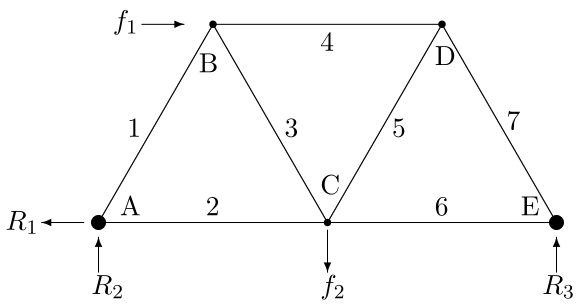
In Figure 2.2.1 we show a truss with equilateral triangles. In Statics you may use the “method of joints” to write equations for each node of the truss 1
See http://en.wikipedia.org/wiki/Truss or http://en.wikibooks.org/wiki/Statics for reference.
. This set of equations is an example of a linear system. Making the approximation \(\sqrt{3}/2 \approx .8660\text{,}\) the equations for this truss are
Figure2.2.1.An equilateral truss. Joints or nodes are labeled alphabetically, \(A\text{,}\)\(B\text{,}\) … and Members (edges) are labeled numerically: \(1\text{,}\)\(2\text{,}\) …. The forces \(f_{1}\) and \(f_{2}\) are applied loads and \(R_{1}\text{,}\)\(R_{2}\) and \(R_{3}\) are reaction forces applied by the supports.
You could solve this system by hand with a little time and patience; systematically eliminating variables and substituting. Obviously, it would be a lot better to put the equations on a computer and let the computer solve it. In the next few sections we will learn how to use a computer effectively to solve linear systems. The first key to dealing with linear systems is to realize that they are equivalent to matrices, which contain numbers, not variables.
As we discuss various aspects of matrices, we wish to keep in mind that the matrices that come up in engineering systems are really large. It is not unusual in real engineering to use matrices whose dimensions are in the thousands! It is frequently the case that a method that is fine for a \(2 \times 2\) or \(3 \times 3\) matrix is totally inappropriate for a \(2000 \times 2000\) matrix. We thus want to emphasize methods that work for large matrices.
The advantage of the augmented matrix, is that it contains only numbers, not variables. The reason this is better is because computers are much better in dealing with numbers than variables. To solve this system, the main steps are called Gaussian elimination and back substitution.
Notice that a lot of the entries are \(0\text{.}\) Matrices like this, called sparse, are common in applications and there are methods specifically designed to efficiently handle sparse matrices.
Recall that each row represents an equation and each column a variable. The last row represents the equation \(2 x_{3} = 4\text{.}\) The equation is easily solved, i.e. \(x_{3} = 2\text{.}\) The second row represents the equation \(- x_{2} + 6 x_{3} = 7\text{,}\) but since we know \(x_{3} = 2\text{,}\) this simplifies to: \(- x_{2} + 12 = 7\text{.}\) This is easily solved, giving \(x_{2} = 5\text{.}\) Finally, since we know \(x_{2}\) and \(x_{3}\text{,}\) the first row simplifies to: \(x_{1} - 10 + 6 = 4\text{.}\) Thus we have \(x_{1} = 8\) and so we know the whole solution vector: \(\xb = \langle 8 , 5, 2 \rangle\text{.}\) The process we just did is called back substitution, which is both efficient and easily programmed. The property that made it possible to solve the system so easily is that \(A\) in this case is upper triangular. In the next section we show an efficient way to transform an augmented matrix into an upper triangular matrix.
The first step of Gaussian elimination is to get rid of the 2 in the (2,1) position by subtracting \(2\) times the first row from the second row, i.e. (new 2nd = old 2nd - (2) 1st). We can do this because it is essentially the same as adding equations, which is a valid algebraic operation. This leads to
There is already a zero in the lower left corner, so we don’t need to eliminate anything there. To eliminate the third row, second column, we need to subtract \(-2\) times the second row from the third row, (new 3rd = old 3rd - (-2) 2nd), to obtain
Set \(f_{1} = 1000N\) and \(f_{2} = 5000N\) in the equations (2.2.1) for the equailateral truss. Input the coefficient matrix \(A\) and the right hand side vector \(b\) in (2.2.2) into MATLAB. Solve the system using the command \ to find the tension in each member of the truss. Save the matrix \(A\) as A_equil_truss and keep it for later use. (Enter save A_equil_truss A.) Print out and turn in \(A\text{,}\)\(\bb\) and the solution \(\xb\text{.}\)
Write each system of equations as an augmented matrix. By hand, find the solutions using Gaussian elimination and back substitution (i.e. the exact algorithm in this section). Check your solutions using MATLAB.