Insulated Boundary Conditions

Section 4.9 Insulated Boundary Conditions

Subsection 4.9.1 Insulation

In many of the previous sections we have considered fixed boundary conditions, i.e. \(u(0) = a\text{,}\) \(u(L) = b\text{.}\) We implemented these simply by assigning \(u_{0}^{j} =a\) and \(u_{n}^{j} = b\) for all \(j\text{.}\)

🔗

We also considered variable boundary conditions, such as \(u(0,t) = g_{1}( t)\text{.}\) For example, we might have \(u(0,t) = \sin( t)\) which could represent periodic heating and cooling of the end at \(x=0\text{.}\)

🔗

A third important type of boundary condition is called the insulated boundary condition. It is so named because it mimics an insulator at the boundary. Physically, the effect of insulation is that no heat flows across the boundary. This means that the temperature gradient is zero, which implies that we should require the mathematical boundary condition \(u'(L) = 0\text{.}\)

🔗

To use it in a program, we must replace \(u'(L) = 0\) by a discrete version. Recall that in our discrete equations we usually have \(L = x_{n}\text{.}\) Recall from the section on numerical derivatives, that there are three different ways to replace a derivative by a difference equation, left, right and central differences. The three of them at \(x_{n}\) would be

\begin{equation*} u'(x_{n}) \approx \frac{u_{n} - u_{n-1}}{h}\approx \frac{u_{n+1}- u_{n}}{h}\approx \frac{u_{n+1}- u_{n-1}}{2 h}\text{.} \end{equation*}

If \(x_{n}\) is the last node of our grid, then it is clear that we cannot use the right or central difference, but are stuck with the first of these. Setting that expression to zero implies

\begin{equation*} u_{n} = u_{n-1}\text{.} \end{equation*}

This restriction can be easily implemented in a program simply by putting a statement u(n+1)=u(n) inside the loop that updates values of the profile. However, since this method replaces \(u'(L) =0\) by an expression that is only accurate to first order, it is not very accurate and is usually avoided.

🔗

Instead we want to use the most accurate version, the central difference. For that we should have

\begin{equation*} u'(L) = u'(x_{n}) = \frac{u_{n+1}- u_{n-1}}{2h}= 0\text{,} \end{equation*}

or simply

\begin{equation*} u_{n+1}= u_{n-1}\text{.} \end{equation*}

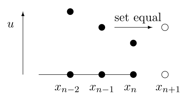
However, \(u_{n+1}\) would represent \(u(x_{n+1})\) and \(x_{n+1}\) would be \(L+h\text{,}\) which is outside the domain. This, however, is not an obstacle in a program. We can simply extend the grid to one more node, \(x_{n+1}\text{,}\) and let \(u_{n+1}\) always equal \(u_{n-1}\) by copying \(u_{n-1}\) into \(u_{n+1}\) whenever \(u_{n-1}\) changes. The point \(x_{n+1}\) is “fictional”, but a computer does not know the difference between fiction and reality! This idea is carried out in the calculations of the next section and illustrated in Figure 4.9.1.

🔗

Schematic of enforcing an insulated boundary condition.🔗 — Figure 4.9.1. Illustation of an insulated boundary condition using a fictional point \(x_{n+1}\) with \(u_{n+1}=u_{n-1}\text{.}\)
🔗

A way to think of an insulated boundary that makes sense of the point \(L+h\) is to think of two bars joined end to end, where you let the second bar be mirror image of the first bar. If you do this, then no heat will flow across the joint, which is exactly the same effect as insulating.

🔗

Another practical way to implement an insulated boundary is to let the grid points straddle the boundary. For example suppose we want to impose insulated boundary at the left end of a bar, i.e. \(u'(0) =0\text{,}\) then you could let the first two grid points be at \(x_{0} = -h/2\) and \(x_{1} = h/2\text{.}\) Then you can let

\begin{equation*} u_{0} = u_{1}\text{.} \end{equation*}

This will again force the central difference at \(x=0\) to be \(0\text{.}\)

🔗

Subsection 4.9.2 Implementation in a linear equation by elimination

Consider the BVP

\begin{equation} u_{xx}= -1\quad\text{with}\quad u(0) = 5\quad\text{and}\quad u'(1) = 0\text{.}\tag{4.9.1} \end{equation}

This represents the steady state temperature of a bar with a uniformly applied heat source, with one end held at a fixed temperature and the other end insulated.

🔗

If we use 4 equally spaced intervals, then

\begin{equation*} m=4\quad\text{and}\quad L=1 \quad \Rightarrow \quad h = \frac{L}{m}= \frac{1}{4} \end{equation*}

and

\begin{equation*} x_{0} = 0,\, x_{1} = .25,\, x_{2} = .5,\, x_{3} = .75,\, x_{4} = 1,\, \text{ and }x_{5} = 1.25\text{.} \end{equation*}

The point \(x_{5} = 1.25\) is outside the region and thus fictional. The boundary condition at \(x_{0} = 0\) is implemented as

\begin{equation*} u_{0} = 5\text{.} \end{equation*}

For the insulated condition, we will require

\begin{equation*} u_{5} = u_{3}\text{.} \end{equation*}

This makes the central difference for \(u'(x_{4})\) be zero. We can write the differential equation as a difference equation

\begin{equation*} \frac{u_{i-1}-2 u_{i} + u_{i+1}}{h^{2}}= -1 \end{equation*}

\begin{equation*} u_{i-1}-2 u_{i} + u_{i+1}= -0.0625, \quad i = 1,2,3,4\text{.} \end{equation*}

For \(i = 1\text{,}\) recalling that \(u_{0} = 5\text{,}\) we have

\begin{equation*} 5 - 2 u_{1} + u_{2} = -.0625 \quad \textrm{ or }\quad - 2 u_{1} + u_{2} = -5.0625\text{.} \end{equation*}

For \(i=2\) and \(i=3\) we have

\begin{equation*} u_{1} - 2 u_{2} + u_{3} = -.0625 \quad \textrm{ and }\quad u_{2} -2 u_{3} + u_{4} = -.0625\text{.} \end{equation*}

For \(i=4\) we have

\begin{equation*} u_{3} - 2 u_{4} + u_{5} = -.0625\text{.} \end{equation*}

Note that we now have 5 unknowns in our problem: \(u_{1}, \ldots, u_{5}\text{.}\) However, from the boundary condition \(u_{5} = u_{3}\) and so we can eliminate \(u_{5}\) from our \(i=4\) equation and write

\begin{equation*} 2 u_{3} - 2 u_{4} = -.0625\text{.} \end{equation*}

Summarizing, we can put the unknown quantities in a vector \(\ub = (u_{1},u_{2},u_{3},u_{4})'\) and write the equations as a matrix equation \(A \ub = \bb\) where

\begin{equation*} A = \left( \begin{array}{cccc}-2 & 1 & 0 & 0 \\ 1 & -2 & 1 & 0 \\ 0 & 1 & -2 & 1 \\ 0 & 0 & 2 & -2\end{array} \right) \end{equation*}

and \(\bb = (-5.0625, -.0625, -.0625, -.0625)'\text{.}\) Solve this system and plot the results:

>> u = A \ b
>> u = [5 ; u]
>> x = 0:.25:1
>> plot(x,u,'d')

Then interpolate with a spline.

🔗

The exact solution of this BVP is:

\begin{equation*} U(x) = 5 + x - .5 x^{2}\text{.} \end{equation*}

Use hold on and plot this function on the same graph to compare:

>> xx = 0:.01:1;
>> uu = 5 + xx - .5*xx.^2;
>> hold on
>> plot(xx,uu,'r')

You should see that our approximate solution is almost perfect!

🔗

Subsection 4.9.3 Insulated boundary conditions in time-dependent problems

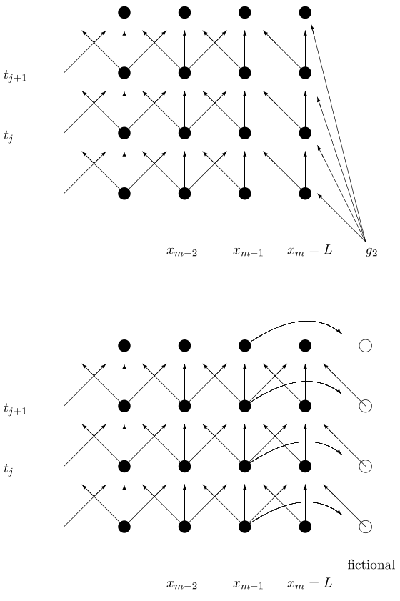
To implement the insulated boundary condition in an explicit difference equation with time, we need to copy values from inside the region to fictional points just outside the region. Note that you copy the new value from inside the region to the false point during each time step, i.e. inside the loop, but after the values are updated at the real points. See Figure 4.9.2 for an illustration.

🔗

Schematic of enforcing a time-dependent insulated boundary condition.🔗 — Figure 4.9.2. Illustration of information flow for the explicit method near the right boundary at \(x=L\text{.}\) The top figure shows a fixed boundary condition, where \(u_{m,j}\) is set to be \(g_{2}(t_{j})\text{.}\) The bottom figure shows an insulating boundary condition. Now \(u_{m,j}\) is updated in the same way as the general \(u_{i,j}\) and an additional entry \(u_{m+1,j}\) is used with its value set by copying \(u_{m-1,j}\text{.}\)
🔗

🔗

Subsection 4.9.4 An example

The steady state temperature \(u(r)\) (given in polar coordinates) of a disk subjected to a radially symmetric heat load \(g(r)\) and cooled by conduction to the rim of the disk and radiation to its environment is determined by the boundary value problem

\begin{equation*} \frac{\partial^{2} u}{\partial r^{2}}+ \frac{1}{r}\frac{\partial u}{\partial r}= d (u^{4} - u_{b}^{4}) - g(r) \quad\text{with}\quad u(R) = u_{R} \quad\text{and}\quad u'(0) = 0\text{.} \end{equation*}

Here \(u_{b}\) is the (fixed) background temperature and \(u_{R}\) is the (fixed) temperature at the rim of the disk.

🔗

The program myheatdisk.m (Program A.2.4) implements these equations for parameter values \(R = 5\text{,}\) \(d = .1\text{,}\) \(u_{R} = u_{b} = 10\) and \(g(r) = (r-5)^{2}\text{.}\) Notice that the equations have a singularity (discontinuity) at \(r=0\text{.}\) How does the program avoid this problem? How does the program implement \(u_{R}=10\) and \(u'(0) = 0\text{?}\) Run the program.

🔗

Exercises 4.9.5 Exercises

1.

Redo the calculations for the BVP (4.9.1) except do not include the fictional point \(x_{5}\text{.}\) Instead, let \(x_{4}\) be the last point and impose the insulated boundary by requiring \(u_{4} = u_{3}\text{.}\) (Keep \(m=4\) and \(h=1/4\text{.}\) Your system of equations should be \(3 \times 3\text{.}\)) Compare this solution with the true solution and the better approximation in the section. Illustrate this comparison on a single plot.

🔗

2.

Modify the program myheat.m (Program 4.6.2) to have an insulated boundary at \(x=L\) (rather than \(u(L,t) = g_{2}(t)\)). You will need to change the domain to: x = 0:h:L+h, change the dimensions of all the other objects to fit this domain and implement the insulation (copy) step inside the loop (see Subsection 4.9.3 and Figure 4.9.2).

🔗

Run the program with \(L = 2\pi\text{,}\) \(T=20\text{,}\) \(c = .6\text{,}\) \(g_{1}(t) = \sin(t)\) and \(f(x) = -\sin(x/4)\text{.}\) Set \(m=20\) and experiment with \(n\text{.}\) Get a plot when the program is stable. Turn in your program and plot.

🔗

Prev Top Next