
Section 4.4 ODE Boundary Value Problems and Finite Differences

Subsection 4.4.1 Steady State Heat and Diffusion

If we consider the movement of heat in a long thin object (like a metal bar), it is known that the temperature, \(u(x,t)\text{,}\) at a location \(x\) and time \(t\) satisfies the partial differential equation
\begin{equation*} u_{t} - u_{xx}= g(x,t)\text{,} \end{equation*}
where \(g(x,t)\) is the effect of any external heat source. The same equation also describes the diffusion of a chemical in a one-dimensional environment. For example the environment might be a canal, and then \(g(x,t)\) would represent how a chemical is introduced.
Sometimes we are interested only in the steady state of the system, supposing \(g(x,t) = g(x)\) and \(u(x,t) = u(x)\text{.}\) In this case
\begin{equation*} u_{xx}= -g(x)\text{.} \end{equation*}
This is a linear second-order ordinary differential equation. We could find its solution exactly if \(g(x)\) is not too complicated. If the environment or object we consider has length \(L\text{,}\) then typically one would have conditions on each end of the object, such as \(u(0) = 0\text{,}\) \(u(L) = 0\text{.}\) Thus instead of an initial value problem, we have a boundary value problem or BVP.

Subsection 4.4.2 Beam With Tension

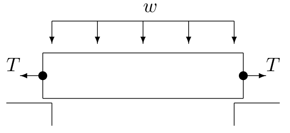
Consider a simply supported beam with modulus of elasticity \(E\text{,}\) moment of inertia \(I\text{,}\) a uniform load \(w\text{,}\) and end tension \(T\) (see Figure 4.4.1). If \(y(x)\) denotes the deflection at each point \(x\) in the beam, then \(y(x)\) satisfies the differential equation
\begin{equation*} \frac{y''}{(1 + (y')^{2})^{3/2}}- \frac{T}{EI}y = \frac{wx(L-x)}{2EI}\text{,} \end{equation*}
with boundary conditions \(y(0) = y(L) = 0\text{.}\) This equation is nonlinear and there is no hope to solve it exactly. If the deflection is small then \((y')^{2}\) is negligible compared to 1 and the equation approximately simplifies to
\begin{equation} y'' - \frac{T}{EI}y = \frac{wx(L-x)}{2EI}\text{.}\tag{4.4.1} \end{equation}
This is a linear equation and we can find the exact solution. We can rewrite the equation as
\begin{equation} y'' - \alpha y = \beta x(L-x)\text{,}\tag{4.4.2} \end{equation}
where
\begin{equation} \alpha = \frac{T}{EI}\quad \text{ and }\quad \beta= \frac{w}{2EI}\text{,}\tag{4.4.3} \end{equation}
and then the exact solution is
\begin{equation} y(x) = \frac{2\beta}{\alpha^{2}}\frac{e^{\sqrt{\alpha}L}}{e^{\sqrt{\alpha}L}+1}e^{-\sqrt{\alpha}x}+ \frac{2\beta}{\alpha^{2}}\frac{1}{e^{\sqrt{\alpha}L}+1}e^{\sqrt{\alpha}x}+ \frac{\beta}{\alpha}x^{2} - \frac{\beta L}{\alpha}x + \frac{2\beta}{\alpha^{2}}\text{.}\tag{4.4.4} \end{equation}

Schematic of a beam.🔗
Figure 4.4.1. A simply supported beam with a uniform load \(w\) and end tension \(T\text{.}\)

Subsection 4.4.3 Finite Difference Method – Linear ODE

A finite difference equation is an equation obtained from a differential equation by replacing the variables by their discrete versions and derivatives by difference formulas.
First we will consider equation (4.4.1). Suppose that the beam is a W12x22 structural steel I-beam. Then \(L = 120\) in., \(E = 29 \times 10^{6} \textrm{lb.}/\textrm{in.}^{2}\) and \(I = 121 \textrm{in.}^{4}\text{.}\) Suppose that the beam is carrying a uniform load of \(100,000\) lb. so that \(w = 120,000/120 = 10,000\) and a tension of \(T = 10,000\) lb.. We calculate from (4.4.3) \(\alpha = 2.850 \times 10^{-6}\) and \(\beta = 1.425 \times 10^{-6}\text{.}\) Thus we have the following BVP:
\begin{equation} y'' = 2.850 \times 10^{-6}y + 1.425 \times 10^{-6}x(120-x), \qquad y(0) = y(120) = 0\text{.}\tag{4.4.5} \end{equation}
First subdivide the interval \([0,120]\) into four equal subintervals. The nodes of this subdivion are \(x_{0} = 0\text{,}\) \(x_{1} = 30\text{,}\) \(x_{2} = 60\text{,}\) …, \(x_{4} = 120\text{.}\) We will then let \(y_{0}, y_{1}, \ldots, y_{4}\) denote the deflections at the nodes. From the boundary conditions we have immediately:
\begin{equation*} y_{0} = y_{4} = 0\text{.} \end{equation*}
To determine the deflections at the interior points we will rely on the differential equation. Recall the central difference formula
\begin{equation*} y''(x_{i}) \approx \frac{y_{i+1}- 2 y_{i} + y_{i-1}}{h^{2}}\text{.} \end{equation*}
In this case we have \(h = (b-a)/n =(120-0)/4= 30\text{.}\) Replacing all the variables in the equation (4.4.2) by their discrete versions we get
\begin{equation*} y_{i+1}- 2 y_{i} + y_{i-1}= h^{2} \alpha y_{i} + h^{2} \beta x_{i} (L-x_{i})\text{.} \end{equation*}
Substituting in for \(\alpha\text{,}\) \(\beta\) and \(h\) we obtain:
\begin{equation*} \begin{split}y_{i+1}- 2 y_{i} + y_{i-1}&= 900 \times 2.850 \times 10^{-6}y_{i} + 900 \times 1.425 \times 10^{-6}x_{i}(120 - x_{i}) \\&= 2.565 \times 10^{-3}y_{i} + 1.2825 \times 10^{-3}x_{i}(120 - x_{i})\end{split}\text{.} \end{equation*}
This equation makes sense for \(i = 1,2,3\text{.}\) At \(x_{1} = 30\text{,}\) the equation becomes:
\begin{equation*} \begin{split}y_{2} - 2y_{1} + y_{0}&= 2.565 \times 10^{-3}y_{1}+ 1.2825 \times 10^{-3}\times 30(90)\\ \Leftrightarrow y_{2} - 2.002565 y_{1}&= 3.46275\end{split}\text{.} \end{equation*}
Note that this equation is linear in the unknowns \(y_{1}\) and \(y_{2}\text{.}\) At \(x_{2} = 60\) we have:
\begin{equation*} \begin{split}y_{3} - 2 y_{2} + y_{1}&= .002565 y_{2} + 1.2825 \times 10^{-3}\times 60^{2}\\ \Leftrightarrow y_{3} - 2.002565 y_{2} + y_{1}&= 4.617\end{split}\text{.} \end{equation*}
At \(x_{3} = 90\) we have (since \(y_{4}=0\))
\begin{equation*} \begin{split} - 2.002565 y_{3} + y_{2}&= 3.46275\end{split}\text{.} \end{equation*}
Thus \((y_{1},y_{2},y_{3})\) is the solution of the linear system:
\begin{equation*} \left( \begin{array}{ccc|c}-2.002565 & 1 & 0 & 3.46275 \\ 1 & -2.002565 & 1 & 4.617 \\ 0 & 1 & -2.002565 & 3.46275\end{array} \right)\text{.} \end{equation*}
We can easily find the solution of this system in MATLAB:
>> A = [ -2.002565 1 0 ; 1 -2.002565 1 ; 0 1 -2.002565]
>> b = [ 3.46275 4.617 3.46275 ]'
>> y = A
To graph the solution, we need define the \(x\) values and add on the values at the endpoints:
>> x = 0:30:120
>> y = [0 ; y ; 0]
>> plot(x,y,'d')
Adding a spline will result in an excellent graph.
The exact solution of this BVP is given in (4.4.4). That equation, with the parameter values for the W12x22 I-beam as in the example, is in the program myexactbeam.m (Program A.2.2). We can plot the true solution on the same graph:
>> hold on
>> myexactbeam
Thus our numerical solution is extremely good considering how few subintervals we used and how very large the deflection is.
An amusing exercise is to set \(T=0\) in the program myexactbeam.m (Program A.2.2); the program fails because the exact solution is no longer valid. Also try \(T=.1\) for which you will observe loss of precision. On the other hand the finite difference method still works when we set \(T=0\text{.}\)

Exercises 4.4.4 Exercises

1.

Derive the finite difference equations for the BVP (4.4.5) on the same domain (\([0,120]\)), but with eight subintervals and solve (using MATLAB) as in the example. Plot your result, together on the same plot with the exact solution (4.4.4) from the program myexactbeam.m (Program A.2.2).

2.

By replacing \(y''\) and \(y'\) with central differences, derive the finite difference equation for the boundary value problem
\begin{equation*} y'' + y' - y = x\quad\text{on $[0,1]$}\quad\text{with}\quad y(0) = y(1) = 0 \end{equation*}
using 5 subintervals. Solve them and plot the solution using MATLAB.

