Subsection3.6.1The gradient of a function of multiple variables
If \(f(x_{1}, x_{2}, \ldots, x_{n})\) is a real-valued function of \(n\) variables, i.e. \(x_{1}\text{,}\)\(x_{2}\text{,}\) …, \(x_{n}\text{,}\) then the gradient of \(f\) is the vector:
where we use the vector notation \(\mathbf{x}= (x_{1}, x_{2}, \ldots, x_{n})'\text{.}\) For example, if \(f(x_{1},x_{2}) = x_{1}e^{-x_1^2-x_2^2+\sin(x_1x_2)}\text{,}\) then
If a differentiable function of multiple variables, \(f\text{,}\) has a maximum or minimum at point \(\mathbf{x}^{*}\text{,}\) then we will have:
\begin{equation*}
\nabla f(\mathbf{x}^{*}) = \mathbf{0}\quad \text{ (the zero vector)}\text{.}
\end{equation*}
Thus one way to locate max or min points for a specific function is to solve \(\nabla f(\mathbf{x}^{*}) = \mathbf{0}\text{.}\) This will often lead to systems of non-linear equations as we encountered in Section 2.6. For example, for \(f(x_{1},x_{2}) = x_{1}e^{-x_1^2-x_.^2+\sin(x_1x_2)}\text{,}\)to attempt to find critical point we would need to try to solve:
That, obviously, is going to be very hard and in fact is impossible using algebra. Thus we will have to use numerical methods to find any maximum or minimum points. The multiple variable Newton’s method that we learned in section Section 2.6 would be one option. In the next section we introduce another common algorithm.
Subsection3.6.3The gradient ascent or descent method
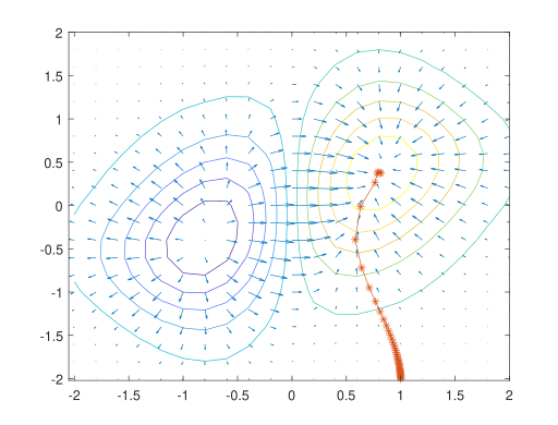
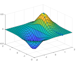
We will take advantage of the fact that the gradient vector points in the direction of greatest increase in the function \(f\text{.}\) If \(f\) is a function of \(x\) and \(y\text{,}\) then we can think of the graph of \(z = f(x,y)\) as a landscape and the gradient points ``uphill’’. That gives us a very handy way to find maximum points, just follow the gradient vectors as they will take you toward higher values of \(z\text{.}\) See Figure 3.6.1.
Since the gradient vector field may change from point to point, we can only ``follow’’ it numerically in finite steps. That is, starting from an initial guess \(\mathbf{x}_{0}\text{,}\) we generate a sequence of points by the formula
The number \(\epsilon\) is often called the ``learning rate’’. It should not be too small or too large. If it is too small the algorithm will be slow. If it is too large, the steps might skip over a critical point. There is ongoing research about how to choose it optimally.
Notice the similarities between this method and the Newton’s method for nonlinear systems in Section 2.6. In both cases we have a function of a vector and generate a sequence of vectors \(\mathbf{x}_{0},\mathbf{x}_{1},\dots\text{.}\)
Find by hand the gradient of the function \(f(x_{1},x_{2}) = \sin(x_{1}) \ e^{-x_1^2 - x_2^2}\text{.}\) Plot it on the rectangle \(-3 \le x_{1} \le 3\text{,}\)\(-2 \le x_{2} \le 2\) using meshgrid and quiver. On the same figure, add the contour plot of \(f\text{.}\)
Write a well-commented script program that uses the gradient descent method to find a minimum point for the function \(f(x_{1},x_{2}) = \sin(x_{1}) \ e^{-x_1^2 - x_2^2}\text{,}\) starting from \(\mathbf{x}_{0} = [-1;-2]\text{.}\) Compare with the plot in Exercise 3.6.4.1 to check that it worked. (Hint: Review the program mymultnewton.m in Section 2.6 for examples of making functions of vectors.)