
Section 3.9 Numerical Differentiation

Subsection 3.9.1 Approximating derivatives from data

Suppose that a variable \(y\) depends on another variable \(x\text{,}\) i.e. \(y = f(x)\text{,}\) but we only know the values of \(f\) at a finite set of points, e.g., as data from an experiment or a simulation:
\begin{equation*} (x_{1},y_{1}), (x_{2},y_{2}), \ldots, (x_{n},y_{n})\text{.} \end{equation*}
Suppose then that we need information about the derivative of \(f(x)\text{.}\) One obvious idea would be to approximate \(f'(x_{i})\) by the Forward Difference
\begin{equation*} f'(x_{i}) = y'_{i} \approx \frac{y_{i+1}- y_{i}}{x_{i+1}-x_{i}}\text{.} \end{equation*}
This formula follows directly from the definition of the derivative in Calculus. An alternative would be to use a Backward Difference
\begin{equation*} f'(x_{i}) \approx \frac{y_{i} - y_{i-1}}{x_{i}-x_{i-1}}\text{.} \end{equation*}
Since the errors for the forward difference and backward difference tend to have opposite signs, it would seem likely that averaging the two methods would give a better result than either alone. If the points are evenly spaced, i.e. \(x_{i+1}-x_{i} = x_{i}-x_{i-1}= h\text{,}\) then averaging the forward and backward differences leads to a symmetric expression called the Central Difference
\begin{equation*} f'(x_{i}) = y'_{i} \approx \frac{y_{i+1}- y_{i-1}}{2h}\text{.} \end{equation*}
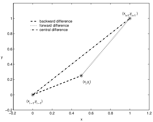
See Figure 3.9.1 for an illustration of these three differences.
Line segments for three difference approximations.
Figure 3.9.1. The three difference approximations of \(y'_{i}\text{.}\)

Subsection 3.9.2 An example

The following code plots the function \(y = \sin(x) + .5\sin(1.5x)\text{,}\) its derivative, and the central difference approximation to the derivative.
>> x = linspace(0,2*pi,51);
>> h = x(2)-x(1);
>> mid = (x(1:end-1)+x(2:end))/2;
>> y = sin(x) + .5*sin(1.5*x);
>> dy1 = (y(2:end)-y(1:end-1))/h;
>> dy2 = cos(x) + .75*cos(1.5*x);
>> plot(x,y,'k',mid,dy1,'b*',x,dy2,'r')

Subsection 3.9.3 Errors of approximation

We can use Taylor polynomials to derive the accuracy of the forward, backward, and central difference formulas. For example the usual form of the Taylor polynomial with remainder (sometimes called Taylor’s Theorem) is
\begin{equation*} f(x+h) = f(x) + h f'(x) + \frac{h^{2}}{2}f''(c)\text{,} \end{equation*}
where \(c\) is some (unknown) number between \(x\) and \(x+h\text{.}\) Letting \(x = x_{i}\text{,}\) \(x+h = x_{i+1}\) and solving for \(f'(x_{i})\) leads to
\begin{equation*} f'(x_{i}) = \frac{f(x_{i+1})-f(x_{i})}{h}- \frac{h}{2}f''(c)\text{.} \end{equation*}
Notice that the quotient in this equation is exactly the forward difference formula. Thus the error of the forward difference is \(- (h/2) f''(c)\) which means it is \(O(h)\text{.}\) Replacing \(h\) in the above calculation by \(-h\) gives the error for the backward difference formula; it is also \(O(h)\text{.}\) For the central difference, the error can be found from the third degree Taylor polynomials with remainder
\begin{align*} f(x_{i+1}) \amp = f(x_{i} + h) = f(x_{i}) + hf'(x_{i})+ \frac{h^{2}}{2}f''(x_{i}) + \frac{h^{3}}{3!}f'''(c_{1}) \quad\text{and}\\ f(x_{i-1}) \amp = f(x_{i} - h) = f(x_{i}) - hf'(x_{i})+ \frac{h^{2}}{2}f''(x_{i}) - \frac{h^{3}}{3!}f'''(c_{2})\text{,} \end{align*}
where \(x_{i} \le c_{1} \le x_{i+1}\) and \(x_{i-1}\le c_{2} \le x_{i}\text{.}\) Subtracting these two equations and solving for \(f'(x_{i})\) leads to
\begin{equation*} f'(x_{i}) = \frac{f(x_{i+1})-f(x_{i-1})}{2h}- \frac{h^{2}}{3!}\frac{f'''(c_{1}) + f'''(c_{2})}{2}\text{.} \end{equation*}
This shows that the error for the central difference formula is \(O(h^{2})\text{.}\) Thus, central differences are significantly better and so: It is best to use central differences whenever possible.
There are also central difference formulas for higher order derivatives. These all have error of order \(O(h^{2})\text{:}\)
\begin{align*} f''(x_{i}) \amp = y''_{i} \approx \frac{y_{i+1}- 2 y_{i} + y_{i-1}}{h^{2}},\\ f'''(x_{i}) \amp = y'''_{i} \approx \frac{1}{2 h^{3}}\left[y_{i+2}- 2y_{i+1}+ 2y_{i-1}- y_{i-2}\right] ,\quad\text{and}\\ f^{(4)}(x_{i}) \amp = y^{(4)}_{i} \approx \frac{1}{h^{4}}\left[y_{i+2}- 4y_{i+1}+ 6y_{i} - 4y_{i-1}+ y_{i-2}\right]\text{.} \end{align*}

Subsection 3.9.4 Partial Derivatives

Suppose \(u = u(x,y)\) is a function of two variables that we only know at grid points \((x_{i},y_{j})\text{.}\) We will use the notation
\begin{equation*} u_{i,j}= u(x_{i},y_{j}) \end{equation*}
frequently throughout the rest of the sections. We can suppose that the grid points are evenly spaced, with an increment of \(h\) in the \(x\) direction and \(k\) in the \(y\) direction. The central difference formulas for the partial derivatives would be
\begin{align*} u_{x}(x_{i},y_{j}) \amp \approx \frac{1}{2h}\left( u_{i+1,j}- u_{i-1,j}\right) \quad\text{and}\\ u_{y}(x_{i},y_{j}) \amp \approx \frac{1}{2k}\left( u_{i,j+1}- u_{i,j-1}\right)\text{.} \end{align*}
The second partial derivatives are
\begin{align*} u_{xx}(x_{i},y_{j}) \amp \approx \frac{1}{h^{2}}\left( u_{i+1,j}-2u_{i,j}+ u_{i-1,j}\right) \quad\text{and}\\ u_{yy}(x_{i},y_{j}) \amp \approx \frac{1}{k^{2}}\left( u_{i,j+1}-2u_{i,j}+ u_{i,j-1}\right)\text{,} \end{align*}
and the mixed partial derivative is
\begin{equation*} u_{xy}(x_{i},y_{j}) \approx \frac{1}{4hk}\left( u_{i+1,j+1}- u_{i+1,j-1}- u_{i-1,j+1}+ u_{i-1,j-1}\right)\text{.} \end{equation*}
Caution: Notice that we have indexed \(u_{ij}\) so that as a matrix each row represents the values of \(u\) at a certain \(x_{i}\) and each column contains values at \(y_{j}\text{.}\) The arrangement in the matrix does not coincide with the usual orientation of the \(xy\)-plane.
Let’s consider an example. Let the values of \(u\) at \((x_{i},y_{j})\) be recorded in the matrix
\begin{equation} (u_{ij}) = \left( \begin{array}{ccccc}5.1 & 6.5 & 7.5 & 8.1 & 8.4 \\ 5.5 & 6.8 & 7.8 & 8.3 & 8.9 \\ 5.5 & 6.9 & 9.0 & 8.4 & 9.1 \\ 5.4 & 9.6 & 9.1 & 8.6 & 9.4\end{array} \right)\tag{3.9.1} \end{equation}
Assume the indices begin at 1, \(i\) is the index for rows and \(j\) the index for columns. Suppose that \(h = .5\) and \(k = .2\text{.}\) Then \(u_{y}(x_{2},y_{4})\) would be approximated by the central difference
\begin{equation*} u_{y}(x_{2},y_{4}) \approx \frac{u_{2,5}- u_{2,3}}{2k}\approx \frac{8.9 - 7.8}{2 \cdot 0.2}= 2.75\text{.} \end{equation*}
The partial derivative \(u_{xy}(x_{2},y_{4})\) is approximated by
\begin{equation*} u_{xy}(x_{2},y_{4}) \approx \frac{u_{3,5}- u_{3,3}- u_{1,5}+ u_{1,3}}{4hk}\approx \frac{9.1 - 9.0 - 8.4 + 7.5}{4\cdot .5 \cdot .2}= -2\text{.} \end{equation*}
Exercises 3.9.5 Exercises

1.

Suppose you are given the data in the following table.
x 0 5 10 15 20
y 0 19 26 29 31
  1. Give the forward, backward and central difference approximations of \(f'(5)\text{.}\)
  2. Give the central difference approximations for \(f''(10)\text{,}\) \(f'''(10)\) and \(f^{(4)}(10)\text{.}\)

2.

Suppose the position of a runner was recorded every half second and the results are given in the following table. Units of distance are meters.
t 0 .5 1.0 1.5 2.0 2.5 3.0 3.5 4.0 4.5 5.0 5.5 6.0
y 0 .25 1 3 6 10 15 21 27 33 39 45 51
Using central differences everywhere possible, and a forward or backward difference where a central difference is not possible, calculate and plot the velocity and the acceleration of the runner as a function of time for \(t=0\) to 6. You may do the calculations by hand or by MATLAB. Turn in your plots and calculations.

3.

Suppose values of \(u(x,y)\) at points \((x_{i},y_{j})\) are given in the matrix (3.9.1). Suppose that \(h = .1\) and \(k = .3\text{.}\) Approximate the following derivatives by central differences:
  1. \(\displaystyle u_{x}(x_{3},y_{4})\)
  2. \(\displaystyle u_{xx}(x_{2},y_{2})\)
  3. \(\displaystyle u_{yy}(x_{3},y_{4})\)
  4. \(\displaystyle u_{xy}(x_{3},y_{3})\)

